Note about the notes
© 2023. This document is licensed under the Creative Commons Attribution-NonCommercial-ShareAlike 4.0 International License.

These notes have been written, edited and published by Oscar Luis Vera-Pérez, using AsciiDoc, AsciiDoctor 2.0.18 and Github Pages. They should be considered as a permanent work in progress. Any constructive feedback is welcome. All errors are ky own.
The initial content of this document was inspired from the (inherited and redefined) conferences taught by Jean-Marc Jézéquel, Yves Le Traon, Benoit Baudry and Benoit Combemale at the University of Rennes. The topics presented in this document have been expanded with content derived from other sources such as the "Introduction to Software Testing" book written by Paul Ammann and Jeff Offutt, "The Fuzzing Book" by Andreas Zeller, Rahul Gopinath, Marcel Böhme, Gordon Fraser, and Christian Holler and the online material on GUI testing published by Tanja Vos. Many other bibliographical sources and materials were also used and appear in the References section. All images from external sources retain their respective copyrights.
As part of the course, students have to complete a set of exercises for each topic. These exercises can be consulted in the following links:
1. Introduction
Software has become omnipresent in our daily lives. Some people even dare to say that “software is eating the world” (1). Nowadays, we depend more and more on the Internet and the Web which are powered by complex interconnected software systems. We trust software to predict the weather, to guard our bank accounts and to order pizza. Through software we communicate with other people and share our photos. We also use streaming services to watch films and listen to music.
Due to its widespread presence there are consequences when software is not properly developed. In some cases, a software glitch has no other repercussion than a hilarious "blue screen of death" in an advertising screen. Sadly, software issues may also cost important amounts of money, they may undermine the reputation of companies and, in some extreme cases, they might even cost human lives.
As developers we need to be sure that the software we build works as expected. This course will briefly introduce some of the most relevant techniques and tools to achieve that goal.
1.1. Bugs, faults, errors and failures
Along with the proliferation of software, the term bug is nowadays known to most people. We say that a software or program has a bug when its behavior produces unexpected results. Bugs may manifest in very different ways, for example, a web page we visit returns an error message instead of the desired content or a character does not jump when we press the right button while playing a video game.
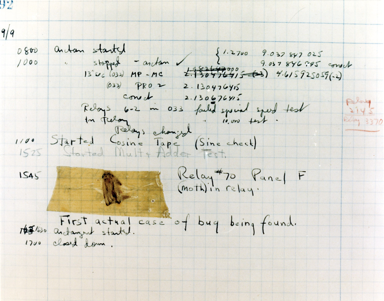
The term bug in Computer Science and Software Engineering has been usually attributed to Grace Hooper. She was involved in the programming and operation of the Mark II, an electromechanical computer of 23 tons and the size of a room. She was also the creator of the first compiler and the only woman to be ranked admiral in the U.S. Navy. Her group traced a computer malfunction to a moth in one of the relays of the machine. This is the first documented case of a computer "bug". The moth was included in one of the notebooks that this group used to log the computer’s operation. It can be seen nowadays at the Smithsonian Institution’s National Museum of American History in Washington D.C Figure 1. However, some historical records state that Thomas Alva Edison already used the term for something similar in his inventions.(2).
Software development usually follows a set of requirements called the product specification. In whatever format it is presented, the specification should describe the features the software will have (functional requirements): e.g.: the program should open a document, save it, the user should be able to change the format and so on. Specifications also include the constraints under which the software should work (non-functional requirement): e.g.: the program should be secure, easy to use and fast (5).
A bug appears when the software does not match the requirements. Maybe the program does not perform correctly a functional requirement e.g. the window closes when the maximize button is pressed or part of a document is not correctly formatted. Also, bugs can make a program violate non-functional requirement e.g. there is a lag between the moment the user types something and the moment the text appears on the screen.
Bugs or faults are produced by human mistakes in the development process. A fault induces a wrong state or error during the execution of the software. When the error produces an incorrect behavior of the program we see a failure.
- Software Fault, Software Defect, Bug
-
Is a manifestation of a human mistake in software. It is a static flaw or imperfection found within the code of a program.
- Software Error
-
An incorrect internal state of the program during execution produced by a fault.
- Software Failure
-
It is a deviation of the software from the expected delivery or service.
A mistake leads to a fault, a fault leads to a software error which leads to a failure when the software is executed. A failure is the manifestation of a bug.
Listing 1 shows a recursive implementation of a binary search over an ordered array. Given an ordered array and a number, the search method returns the position of the number in the array or -1. The private overload of the method uses two auxiliary parameters to delimit the slice of the array that is inspected on each call. The initial slice is the entire array. When the method is invoked, it compares the element in the middle of the slice with the number given as input. If they are equal, then the position in the middle is returned, otherwise the method is invoked with the first half or the second half of the slice. The procedure continues until the number is found in the array, or when there is evidence that the number is not contained, under the assumption that the array is initially sorted.
public static int search(int[] array, int element) {
  return search(array, element, 0, array.length - 1);
}

private static int search(int[] array, int element, int first, int last) {
  if(last < first) {
    return -1;
  }
  int middle = (first + last)/2;
  int median = array[middle];
  if(element == median) {
    return middle;
  }
  if(element < median) {
    return search(array, element, first, middle - 1);
  }
  return search(array, element, middle, last); (1)
}| 1 | This line contains a fault. The correct code should invoke search with middle + 1 instead of middle. |
This implementation has a fault. The second recursive invocation of search: search(array, element, middle, last) should use middle + 1 instead of middle. This fault does not always produce an error. For example, search(new int[]{0, 6, 8, 10}, 6) produces the right result. However, search(new []{0, 6, 8, 10}, 10), leads to an invocation where first=2 and last=3. For this invocation middle, which is computed as (first + last) / 2 results in middle=2. Once the comparisons are done, the same method is invoked again with the same parameters. This is not the right program state and thus it becomes the error produced by the initial fault. As the method is invoked again with the same parameters, it produces an infinite recursion that is manifested through a stack overflow exception. The exception becomes the failure that evidences the initial fault.
Failures may come from all sorts of errors. Some of them could be traced to a very localized and specific part of the code, as in the example before. These are considered as local bugs. Others may be encountered at the interaction of different components of the system. These are considered as global bugs. The following sections describe some famous local and global bugs.
1.1.1. Local bugs and some famous cases
Local bugs can be traced to very specific locations in the code. They can be originated from multiple types of errors such as:
-
Omission of potential cases e.g. not considering that negative numbers could be used in certain operations.
-
Lacks of checks e.g. the code does not verify whether a given parameter is
nullor that divisor must a number different from zero. -
Wrong conditions e.g. using the wrong comparison operator when comparing two numbers.
-
Wrong approximations e.g. wrong values due to type conversions when we convert a
doubleto anintand loose precision.
In the next sections we present some famous local bugs and briefly inspect their causes.
The case of Zune
Zune 30, was released to the public in November 2006. It was the first portable media player released by Microsoft. Suddenly, on December 31st 2008, all Zune devices hung and stopped working. The problem was traced back to a piece of code in the firmware equivalent to Listing 2.
while (days > 365) {
    if (IsLeapYear(year)) { (1)
        if (days > 366) {   (2)
            days -= 366;    (3)
            year += 1;      (4)
        }
    }
    else {
        days -= 365;
        year += 1;
    }
}| 1 | On December 31st, 2008 the value of year was 2008 and the value of days was 366 so isLeapYear(year) evaluated to true. |
| 2 | Since the value of days was 366 days > 366 evaluated to false. This is the fault, it should have been >=. |
| 3 | This is not executed, therefore the value of days does not change. |
| 4 | This is not executed, therefore the value of year does not change. |
The values of days and years did not change which produced a wrong internal state and thus the error. The software enters an infinite loop and the devices became non-responsive.
By the next day, days would be 367 and the code would run perfectly. So Zune devices stop working on December 31st of every leap year. The problem could have been found if the code was tested with the right input date before releasing the product.
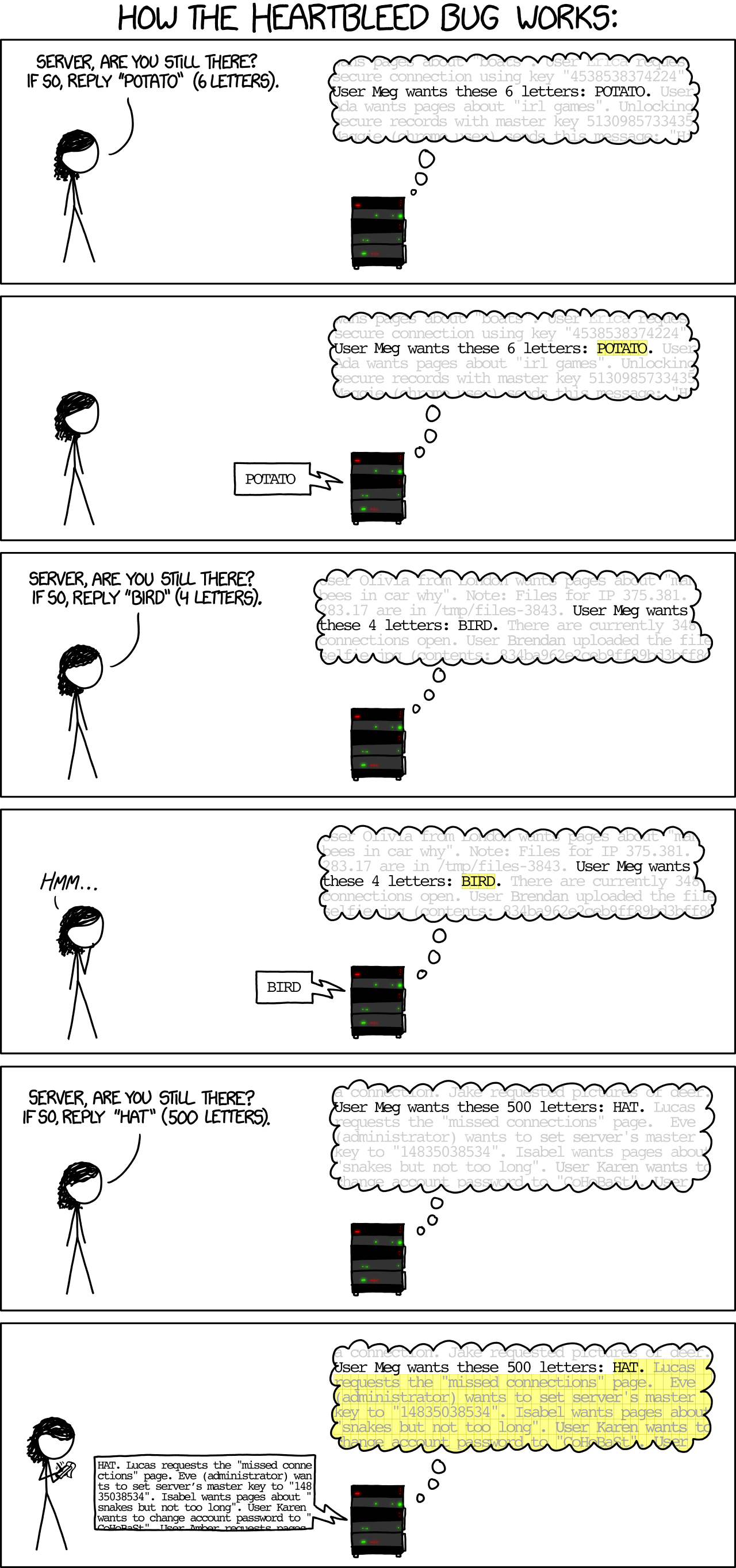
Heartbleed
Heartbleed is a software vulnerability disclosed in April 2014 that granted attackers access to sensitive information. It was caused by a flaw in OpenSSL, an open source code library implementing the Transport Layer Security and Secure Sockets Layer protocols.
As part of these protocols, a computer should send a heartbeat, an encrypted message that the receiver should replay back, to keep the connection alive. The heartbeat contains information about its own length. The code for the receiver never verified that the message had the specified length. To answer, it should allocate a memory buffer to store the content of the heartbeat. If the message was longer, then there is a buffer overflow and the computer would send more data than requested (7).
In Listing 3 you can see a fragment of the code containing the bug.
...
n2s(p, payload); (1)
...
buffer = OPENSSL_malloc(1 + 2 + payload + padding); (2)
bp = buffer;
...
memcpy(bp, pl, payload); (3)
...
s->msg_callback(1, s->version, TLS1_RT_HEARTBEAT,  (4)
	buffer, 3 + payload + padding,
s, s->msg_callback_arg);| 1 | Read payload length into payload. |
| 2 | Allocate memory using the value from the received message. |
| 3 | Copy the payload and potentially sensitive extra information as payload might be larger than what is really required. |
| 4 | Send the data back. |
Other interesting examples
The USS Yorktown (CG-48) cruiser was selected in 1996 as the testbed for the Smart Ship program. The ship was equipped with a network of several 200 MHz Pentium processors. The computers abroad the ship ran Windows NT 4.0 and executed applications to run the control center, monitor the engines and navigate the ship. In September 21st 1997 a crew member entered a zero into a database field causing a division by zero that resulted in a buffer overflow, which, in turn, made the propulsion system fail. The ship was dead for several hours and had to be towed back to port (8).
The Patriot missile defense system was able to track the trajectory of enemy projectiles and intercept them. The system stored the clock time in an integer that was converted to a fixed point number and multiplied by 1/10 to produce the time in seconds for the tracking estimation. The computation was performed in a 24-bit fixed point register and the time value was truncated. This would produce an error proportional to the uptime of the system (i.e. it grows in time). Apart from that, the system was updated several times to improve the conversion routine, but the patch was not placed in all the required code locations. On February 25th, 1991 one of these Patriot batteries failed to intercept an Iraqi Scud missile. The battery had been up for 100 hours and the chopping error was around 0.34 seconds. Since a Scud travels at 1.676 m/s it reaches more than a half kilometer in this time. The Scud struck an American Army barracks killing 28 soldiers and injuring around 100 other people (9).
The Chemical Bank deducted by error about $15 million from more than 100000 customers in one night. The problem was caused by a line of code that should not be executed until further changes were made to the system. This line sent a copy of every ATM transaction to the machine processing paper checks so, all transactions were deducted twice (10).
1.1.2. Global bugs and famous cases
Rather than coming from a specific and localized error, some failures may emerge from the interactions of the modules that compose a system. This evidences that the whole is more than the mere sum of its parts.
Some sources of global bugs could be:
-
Wrong assumptions about third party components.
-
Errors in the reuse of code. For example, using the code in an environment or an architecture for which it was not designed.
-
Concurrency bugs, that lead to race conditions and deadlocks by incorrectly assuming certain order of execution.
-
Improbable or unforeseen interactions between hardware, software and users.
Race conditions and the Northeast blackout of 2003
A race condition appears when the output of a system depends on the sequence or timing of other uncontrollable events. This may lead to a bug when the effects of this assumption are not carefully considered. For example, in a multithreaded application, a piece of code may be (wrongly) assumed to run before another.
The code in Listing 4 shows a simplified example of a race condition.
public class SimpleApplet extends Applet {

    Image art;
    public void init() { (1)
        art = getImage(getDocumentBase(), getParameter("img"));
    }

    public void paint(Graphics g) { (2)
        g.drawImage(art, 0, 0, this); (3)
    }

}| 1 | init initializes art, if it is not invoked, then art is null. |
| 2 | paint could be invoked before invoking init. |
| 3 | If paint is invoked before init art is null which produces an error in this line. |
To prevent this race condition, the code of paint should not assume that art will always point to an instance. To deal with this race condition it is enough to check if art is null or not.
On August 14th, 2003 the alarm of FirstEnergy, an electric utility in Akron, Ohio, should have alerted about an overload in the electricity transmission lines. A race condition stalled the alarm and the primary sever went down. A backup server started processing all demands and also went down after 13 minutes. With both servers down, the information being shown in the screens passed from a refresh rate of 1 to 3 seconds to 59 seconds. The operators were not aware of the actual condition of the grid and the system collapsed affecting an estimated of 50 million people.
| You may find an image circulating the Internet that is supposed to show a satellite view of this blackout. The image is in fact fake or was perhaps edited to show the extension of the affected area. |
Ariane 5
The Ariane 5 test launch is one of the most referenced examples of the impact that a software bug can have. On June 4th 1996, the rocket was launched by the European Space Agency from the French Guiana. After 40 seconds the rocket exploded at more than 3700 meters of altitude.
In (11) the authors explain that, before liftoff, certain computations are performed to align the Inertial Reference System (SRI). These computations should cease at -9 seconds from the launching sequence. But, since there is a chance that a countdown could be put on hold and because resetting the SRI could take several hours, it was preferable to let the computation proceed than to stop it. The SRI continues for 50 seconds after the start of flight mode. Once the rocket is in the air this computation is not used anymore. However, it caused an exception which was not caught and produced the explosion of the rocket.
Part of the software of Ariane 5 was reused from Ariane 4. The later used 16-bit floating point numbers, while the former used 64-bit arithmetic. The conversion of a greater value caused the exception. The fact that this module used 16-bit floating point numbers was not documented in the code. The trajectory of Ariane 5 differed from that of Ariane 4. The former had considerably higher horizontal velocities that produced values above the initial range. This was the first launch after a decade of development with an estimated cost of US$7 billion plus the rocket and cargo were estimated in US$500 million.
The Mars Climate Orbiter
The Mars Climate Orbiter probe crashed when entering the orbit of Mars. The cause was tracked to the fact that one development team was using the International System of Units (meters and kilometers) while another team was using the Imperial Unit System (miles and yards). The loss was estimated in US$235.9 million (12). The subject is still inspiration of many memes cruel jokes.
1.2. Why is it so hard to build correct software?
Software inevitably fails. The causes for this are widely varied as we have seen from the previous examples. No domain related to software escapes from this fact. A failure can have multiple consequences from banal to terrible. But why is it to hard to build correct software?
First of all, programs are very complex artifacts, even those we may consider simple or trivial.
Consider the code presented in Listing 5.
void alert(int n) {
  countdown(n);
  soundAlarm();
}

void countdown(int n) {
  while(n > 1) {
    if (n % 2 == 0)
      n = n /2;
    else
      n = 3 * n + 1;
  }
}
Is it possible to show that the alarm will sound for every value of n?
For this particular example one could attempt to devise a formal proof. But good luck with that! Mathematicians have been trying to do it since 1937 with no success. countdown is, in fact, an implementation of what is known as the Collatz conjecture.
One could also try to verify the program for every possible input, but this is impossible in the general case.
For this particular example, let us assume that n is a 32-bits unsigned integer, then we have 232 possible inputs, that is 4294967296 cases for a very simple code of barely 7 lines of code. If the computation of every input takes on average 2.78e-06 seconds, then we will spend 3 hours finding out the result, if the function stops for every input. 3 hours for barely 7 lines of code!
Determining if a procedure halts when given a specific input is known as the Halting Problem (14). The general case of this problem is undecidable. This means that, in general, we can not known for a given procedure if it will halt when processing a given input.
Let’s prove it. Suppose that it is possible to write a function halts that tells whether a given function f halts when given an input x. That is, halts returns true if f(x) halts (Listing 6) and false otherwise.
f and an input x for f, returns true if the invocation of f(x) halts.function halts(f, x):
...If the halts function exists, then we can create a procedure, confused, that will loop forever if halts returns true (Listing 7).
halts(f, f) is true, otherwise it does halt.function confused(f) {
if (halts(f, f)) (1)
while (true) {}
else
return false;
}If we try to compute confused(confused), halts(f, f) is equivalent to halts(confused, confused). If this evaluates to true, then it means that confused(consfused) halts, but then the procedure enters in an infinite loop and so, in fact, confused(confused), which is what we are evaluating in the first time, does not halt. On the other hand, if the condition is false, it means that confused(confused) does not halt, but then, the procedure halts.
Therefore, confused(confused) halts if and only if confused(confused) does not halt, which is a contradiction, so halts can not exist. This means that, in the general case, we can not prove that a program will halt when processing a given input. Of course, there are specific cases in which this is possible, but it can not be done for all existing procedures.
Proving the correctness of a program is a very difficult task. There are formal methods to try to achieve this, but they rely on mathematical models of the real world that might make unrealistic assumptions and, as abstractions, are different from the real machines in which programs execute.
Software is, of course, much more complex than the small functions we have seen so far. As an example, notice that the number of lines of code has increased exponentially in time (though not always in sync with the complexity of the task that the program should achieve), just take a look at the following comparison:
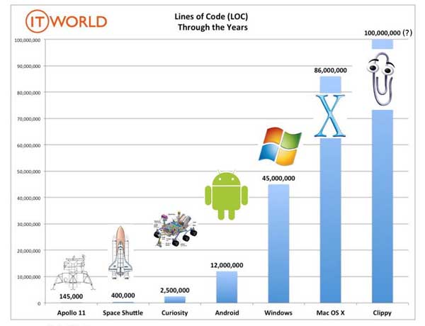
The software of the Apollo 11 Guidance Computer had 145,000 lines of code, while NASA’s Curiosity rover was programmed with 2.5M lines of code. The infamous Clippy on the other hand, had more than 100M lines of code.
Projects such as the Linux Kernel, have triplicated their size in 10 years:
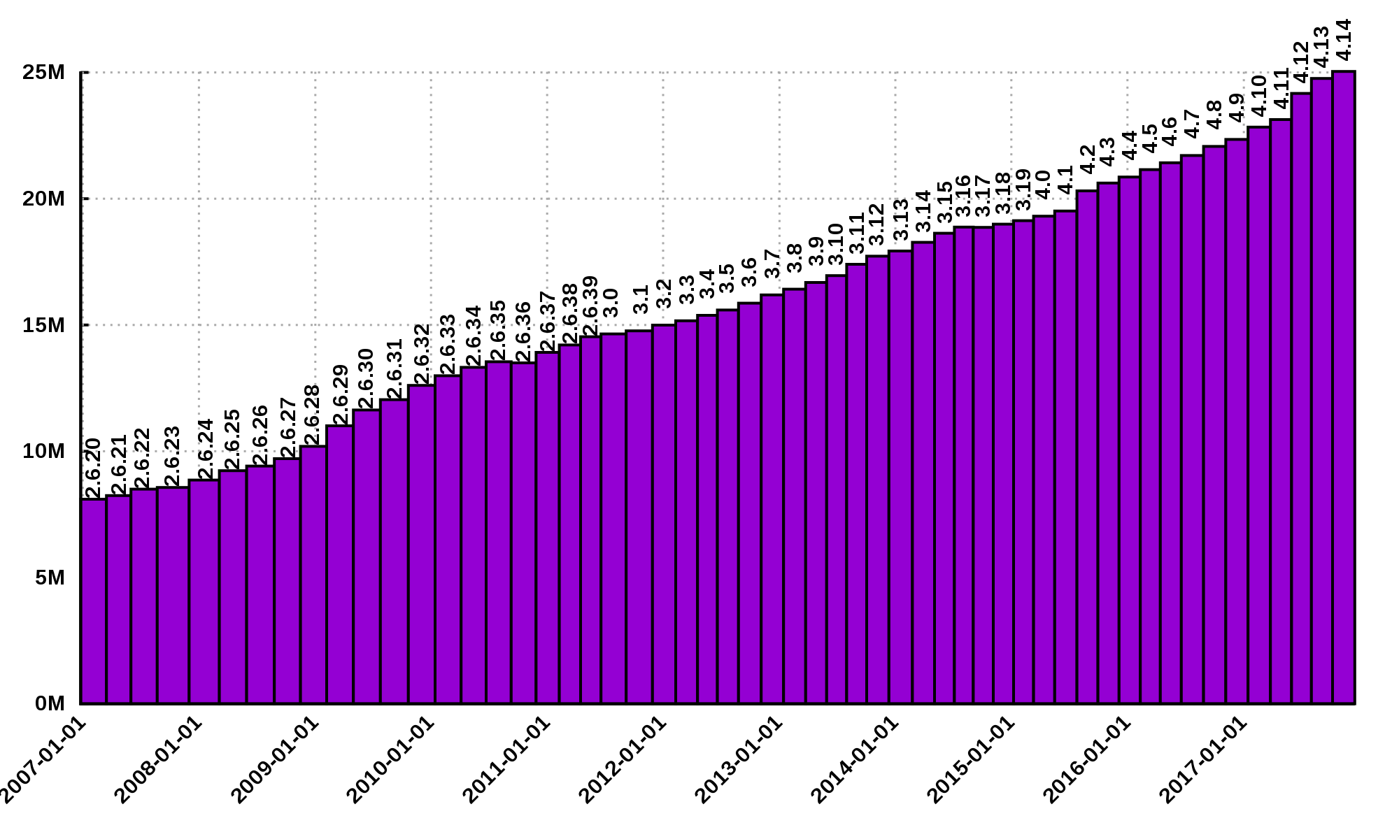
Firefox contains more than 36M lines of code and Chromium more than 18M. More statistics can be found here.
The complexity of software does not come only from its size. For example, in both, Firefox and Chromium developers use more than 15 different programming languages at the same time.
Open source software also grows in complexity as the number of contributors increases. The Firefox project, for example, have had 6477 contributors and 996214 commits as of February 2018.
Also, most software is expected to run in multiple execution platforms, (including hardware, operating system, …). Probably the most dramatic scenario in this sense comes from the mobile world. By August 2015 the OpenSignal company reported the existence of 24,093 different Android devices from 1294 distinct brands (16). Android applications are expected to run correctly in all of them.
Software is also present in systems with real-time computing constraints and sometimes implementing critical functionalities. For example, mp3 players, microwave ovens, GPS devices, medical equipment for vital sign monitoring, avionics (inertial guiding systems), automobiles, fire security systems and the list may go on. As a side note, a car nowadays contains more than 100M lines of code (mostly devoted to the entertainment system), and hundreds of electronic control units (ECU).
On top of that, software is not a static artifact that we release in production and leave as it is. It needs to be maintained over time. For example, Windows 95, was released to manufacturing on August 15th, 1995, it latest release was published on November 26th 1997. However, its mainstream support ended on December 31st, 2000 while the extended support ended on December 31st, 2001, that is five and six years after its latest release. On its side, Windows 7 was released to manufacturing in July 22nd, 2009, support ended on January 14th, 2020 and the extended support for professional users should end on January 10th 2023 while most of us are not using it nowadays.
The COBOL language appeared in 1959. It was estimated that, in 1997, around 80% of business transactions ran in COBOL. Even today, it is even said that more than 220 billions lines of COBOL are in use (17). Migrating these legacy systems may be risky. In 2012 the Commonwealth Bank of Australia replaced its core banking platform to modernize their systems. The change ended up costing around 750 million dollars, which is why many banks have opted to keep their COBOL systems working. Today there are 75-, 60-years-old consultants providing support for COBOL systems in banks (18). In the recent Covid-19 crisis, the state of New Jersey in the U. S. requested COBOL programmers to deal with the 40-years old system to handle the huge amount of unemployment claims they received (19).
The software development process itself could be sometimes rather complex. There are many methodologies about how to build software, and they could even change during the creation of a new product.
So, the complexity of software may come from its requirements, its size as it can be huge, the number of technologies involved on its development as tens of languages and frameworks can be used at the same time, the number of people working on its implementation that could even be hundreds, the diversity of platforms in which it must run and even the development process.
1.3. How to build reliable software?
This is a difficult question and there is no easy answer. Systematically validating and verifying software as it is being built and maintained can lead to fewer bugs. Verification is the process in which we answer Are building the product right?, that is if the software conforms to its specification. Validation answers Are we building the right product?. In this sense we check that the implemented product meets the expectation of the user i.e., whether the specification captures the customer’s needs.
There are three main general approaches to construct reliable software:
- Fault-tolerance
-
Admits the presence of errors and enhance the software with fault-tolerance mechanisms.
- Constructive approach
-
Involves formal modeling. It guarantees the reliability and correctness by construction.
- Analytical approach
-
Involves techniques to analyze the program in order to detect and fix errors.
1.3.1. Fault-tolerance
This approach assumes that it is impossible to prevent the occurrence of bugs in production. So, it enhances the system with mechanisms to deal with them.
N-version programming is an example of this approach. With an initial and rigorous specification, two or more versions of the same system are developed by different development teams (usually with different backgrounds, and using different tools and methods to build the system). In production, these versions are executed in parallel. The actual output of the entire system is an agreement of the results obtained from all versions.
Another example is Chaos engineering popularized by Netflix with its Simian Army. The main concept is to perform a controlled experiment in production to study how the entire system behaves under unexpected conditions. For example, in Netflix, they would simulate random server shutdowns to see how the system responds to this phenomenon (24). This is a form of testing in production. Main challenges are to design the experiments in a way that the system does not actually fail and to pick the system properties to observe. In the case of Netflix, they want to preserve the availability of the content even when the quality has to be reduced.
Finally, approximate computing techniques (20) can be also applied to deal with a trade-off between accuracy and performance in a changing environment (e.g., time-varying bandwidth), when a good enough result is better than nothing (21). For example, Loop Perforation (22), which transforms loops to perform fewer iterations than the original loop, is used to keep the system running in a degraded environment, with a good enough result (e.g., dynamically adapting the video quality according to the actual bandwidth).
1.3.2. Constructive approach
This approach tries to guarantee the absence of bugs by construction. It involves the manual or automatic formal proof of all the components of the system, and their final integration. It is usually based on logical modeling and reasoning and it is used on specific parts of critical software.
The constructive approach may use tools such as Coq, a system to express assertions and mechanically check formal proofs or Isabelle an interactive theorem prover. Listing 8 shows how to use Coq to proof that the depth of any interior node in a tree is greater than 0.
Module TreeExample.

  Inductive tree : Type := (1)
  | Leaf : tree
  | Node : tree -> tree -> tree
  .

  Check Node.

  Definition small_tree : tree := (2)
    Node (Node Leaf Leaf) Leaf.

  (* small_tree tree looks like:
          x
         / \
        x   x
       / \
      x   x
   *)

  Definition is_leaf (t : tree) : bool := (3)
    match t with
    | Leaf => true
    | Node x y => false
    end.

  Fixpoint depth (t : tree) : nat := (4)
    match t with
    | Leaf => 0
    | Node l r => S (max (depth l) (depth r)) (* Succesor of the  *)
    end.

  Lemma depth_positive : (5)
    forall t : tree, 0 < depth t \/ is_leaf t = true.
  Proof.
    induction t.
    {
      cbv [depth is_leaf]. (6)
      right. (7)
      reflexivity. (8)
    }
    {
      cbn [depth is_leaf]. (9)
      left. (10)
      lia. (11)
    }
Qed.| 1 | Definition of a tree type. |
| 2 | Creating an instance of tree with three leaves and two intermediate nodes. |
| 3 | Defining is_leaf which tells whether the given tree is a leaf or not. |
| 4 | Defining a function to compute the depth of a leaf. |
| 5 | Defining a lemma stating that the depth of a tree is positive when the tree is not a leaf. |
| 6 | Inline definitions for depth and is_leaf. |
| 7 | Set the right part of the disjunction as goal for the proof. |
| 8 | The right part is true. This proves true = true. |
| 9 | Inline again, but do not overwrite depth and is_leaf. This avoids recursive calls to depth. |
| 10 | Set the left part of the disjunction as the goal. |
| 11 | According to depth, the node can not be a leaf. So the second part of the depth definition is used. This is the inductive step. The successor of a natural number is always greater than 0. |
The Coq system helps mechanizing the proof of lemmas and theorems by identifying the facts that can be used to achieve the proof and the formulas that still need to be proven.
Coq is also able to extract executable programs from definitions and theorems. There are additional extensions and tools to apply this methodology to other programming languages.
CompCert is the first formally verified C compiler, but it is not bug-free even when a lot of effort has been invested into its formal verification. As said before, the main problem with formal proofs comes from the assumptions they make to abstract the real world. The following quote explains the reason behind a bug found in CompCert:
The problem is that the 16-bit displacement field is overflowed. CompCert’s PPC semantics failed to specify a constraint on the width of this immediate value, on the assumption that the assembler would catch out-of-range values. In fact, this is what happened. We also found a handful of crash errors in CompCert.
Constructive approaches may also involve a form of model checking. These approaches represent the system as a formal behavioral model, usually transition systems or automata. The verification of these models is made with an exhaustive search on the entire state space. The specification of these models are written with the help of logic formalisms. The exhaustive search is directed to verify properties the system must have, for example, the absence of deadlocks. Model checking is used in hardware and software verification and, in most cases, they are performed at the system level. They find application in defense, nuclear plants and transportation.
The following diagram shows a model of the functioning of a microwave oven as a Kripke structure. (Adapted from https://www.dsi.unive.it/~avp/14_AVP_2013.pdf). The model includes first order propositions that characterize the states of the system and a transitional relationship between the states.
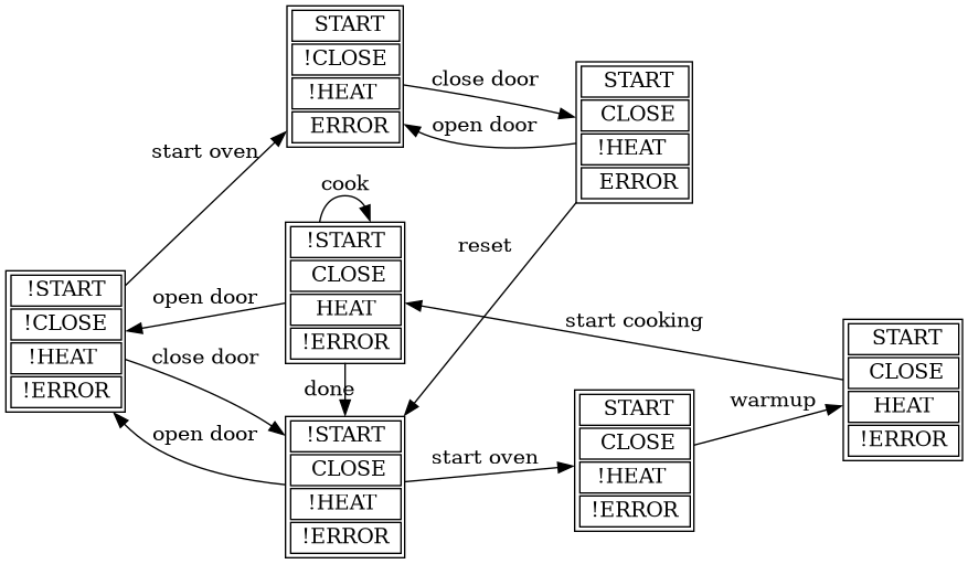
These models can be used to generate concrete code that, for example, would be embedded in specific hardware, and it is possible to verify the state of the system at random inputs and even prove or falsify properties, e.g. for every input the heat is not on while the door is open.
1.3.3. Analytical approach
This approach is directed to find the presence of bugs in the system. It is regularly based on heuristics and can target all kinds of software artifacts: code, models, requirements, etc. Its more used variant is software testing which evaluates a program by observing its execution under different conditions [ammann2017introduction]. Testing presents, nowadays, the best trade-off between effort and result when it comes to the verification and validation of a software product. It will be the main focus of this course.
Bertrand Meyer proposes seven principles of testing (23):
- Principle 1: To test a program is to try to make it fail
-
This is the main purpose of testing, to find defects in the code. In the words of Meyer the single goal of testing is to uncover faults by triggering failures. Testing can not be used to show the absence of bugs, as Dijkstra said and Meyer recalls. But it is extremely useful in finding those scenarios in which the software does not behave as intended. This definition of Meyer presents testing as a dynamic technique, that is, testing requires the execution of a program. However, there are some static code analysis techniques and tools that help detecting potential faults by finding well known code patterns that are prone to errors, or that ensure code quality by forcing development guidelines. In the long term these techniques help reducing the occurrence of bugs at a lower cost, since they don’t execute the program. Some authors refer to these analyses as static testing. There is controversy on whether these static analyses are in fact testing or not, but since they are highly valuable for the quality of the software we shall discuss them in the course.
- Principle 2: Tests are no substitute for specifications
-
Tests are built from specific cases, instances of the different scenarios in which the software shall execute. The specification is composed of more general abstractions tied to human understanding. While the specification can be used to derive test cases the opposite is not necessarily true. Even in large numbers, a finite amount of tests may not capture the general properties of the system due to missing instances.
- Principle 3: Any failed execution must yield a test case, to remain a permanent part of the project’s test suite
-
Once a fault has been discovered there is always the peril that it can reappear later. It happens often in practice. Uncovered faults should then become test cases that prevent these regressions. This is known as regression testing.
- Principle 4: Determining the success or failure of tests must be an automatic process
-
Once a test is executed, one needs to know if the software behaved as expected. Thus, we need a test oracle to produce such verdict. As the number of test cases grows, this task must be automated. It does not scale to run hundreds of test cases, print the output of the program and then manually check whether the output is correct.
- Principle 5: An effective testing process must include both manually and automatically produced test cases
-
Manually produced test cases come from the understanding developers have about the problem domain and the input, or from Principle 3, as Meyer explains. But often corner and specific cases escape from human intuition. Complementing manually designed test cases with automatically produced test cases can help spot what developers missed. Computers are able to generate test cases to a level that humans can not reach and help explore unforeseen scenarios.
- Principle 6: Evaluate any testing strategy through objective assessment using explicit criteria in a reproducible testing process
-
Any testing strategy must be assessed empirically. No matter how sophisticated a testing technique can be, it is of no use if it can not discover faults. Meyer recalls that simple techniques such as random testing are proven to be quite efficient. Then there is the question on how to evaluate the effectiveness of our testing strategy.
- Principle 7: A testing strategy’s most important property is the number of faults it uncovers as a function of time
-
Code coverage, that is, the parts of the code executed in the test cases is often used to evaluate the quality of tests. However, this is only useful to spot the parts of the code that aren’t yet tested, not how well the executed parts are verified. So, coverage is not, in general, a measure of the quality of the tests. The assessment of the tests should correspond to their ability to detect bugs. In this principle Meyer includes time. Of course, the faster faults are encountered, the better.
This set of principles is not comprehensive and not all authors and practitioners agree with all aspects of their formulations. However, in our opinion, they reveal the essence of testing.
| Meyer’s article Seven Principles of Software Testing provoked an answer from Gerald D. Everett, a testing expert and also author of books on the topic. The answer qualified Meyer’s principles as insufficient since they don’t encompass other software quality aspects. The discussion went on with more answers and short essays from both authors. The entire discussion is worth the reading. More details and pointers can be found in Meyer’s own blog: https://bertrandmeyer.com/2009/08/12/what-is-the-purpose-of-testing/. Needless to say, we agree with Meyer’s point of view. |
1.3.4. Modern practices: CI/CD and DevOps
Nowadays testing is automated as much as possible. Software developers use automated processes to facilitate the integration of the work done separately by team members, detect errors as fast as possible and automate most tedious and error-prone tasks.
Continuous Integration (CI) is one of those practices. It is a process in which developers frequently integrate their code into a single shared source control repository. After a change is pushed to a central repository, an automated pipeline is triggered to build and verify the application after the incorporation of the new change. (25) (26)
According to Martin Fowler:
Continuous Integration doesn’t get rid of bugs, but it does make them dramatically easier to find and remove.
Chief Scientist ThoughtWorks
The frequent integration of each developer’s work facilitate the early detection of errors as opposed to each developer working on isolation and then spending a lot of time dealing with the combination of their individual efforts. Most software companies these days use a form of CI and the most used source control hosting services such as Github, Gitlab and Bitbucket encourage these practices by making it easy to incorporate CI tools and even providing their own CI automation alternatives.
According to Thoughtworks, (26) CI processes are supported by the following practices:
- Maintenance of a single source repository
-
All team members should merge their changes into a global/unique code repository, hosted in a source control hosting service, either in-premises or using a public service like Github. The source control repository plays an important role in the identification of a change and the detection of conflicts between simultaneous changes. The common practice nowadays is to use distributed source control systems like Git of Mercurial in opposition to the previous centralized systems like CVS or SVN. Even when the source control system is distributed, that is, every developer has a copy of the repository, the CI process should monitor one central repository to which all developers should push their changes. This does not exclude the creation of mirror repositories.
- Automate the build
-
Once a developer pushes her changes into the global repository, a CI server checks out the changes and triggers a build process. This build process is expected to be self-testing, that is, as part of the automated build, tests should be executed to verify the changes in the code. These tests should also be executed in an environment as close as possible to the production conditions. The build is also expected to be fast so developers have a quick feedback on the change they integrated and the outcome of the build process should be accessible to all team members so they know the current state of the project.
CI processes also impose responsibilities to developers as they are expected to push changes frequently. Also changes should be tested before integrating them into the global repository. Also, developers should not push any change while the automated build fails, that is, when a previous change produced a failure in the CI build process either compiling or running the tests. When a build fails it should be fixed as fast as possible to ensure the quality of the integrated code in the global repository.
CI processes are often accompanied by Continuous Delivery and Continuous Deployment processes.
Continuous Delivery is an automated process involving a verification pipeline whose outcome determines if a change is ready to be deployed. It may involve a larger build process than the one of the CI, including acceptance tests, which are tests in direct correlation to the requirements or the user’s needs, tests in several environment conditions, such as different operating systems, and it may even include manual testing. Once a change passes the delivery pipeline it is considered as robust enough to be deployed.
On its side, Continuous Deployment is an automated process to set artifacts produced and verified by successful builds into production. Continuous Deployment requires Continuous Delivery. Both enable frequent product releases. Some companies may release their products in a daily or even an hourly basis.
CI/CD approaches find great realization in DevOps. DevOps is a modern development culture in which team members of all roles commit to the quality of the final product and not just divide themselves into silos like the "development team" or "operation team". Automation is at the core of DevOps as every development phase is backed by automated processes and state-of-the-art tools. In DevOps, all phases: plan, code, build, test, release, deploy, operate, monitor are imbricated in an infinite loop (Figure 6) and the outcome of one phase impacts the other. For example, crashes observed in production by monitoring the system, automatically become an issue for developers and are incorporated to the set of tests.

2. Code quality and static analysis
The goal of any software project is to deliver a product of the highest possible quality, or at least it should be. Good software has scarce bugs. However, the notion of quality also characterizes how the product is being built and structured. Observing these aspects should help, in the end, to avoid the introduction of bugs. Diomidis Spinellis in his book Code Quality: The Open Source Perspective (26) presents four views of software quality:
- Quality in use
-
This view is centered in the user experience (UX), that is, how users perceive the software. It is the extent to which users can achieve their goals in a particular environment. It does not care about how the product is built. If a word processor makes it hard to edit a document, then it does not serve it purposes.
- External quality attributes
-
These attributes manifest themselves in the execution of the program. They characterize how well the product conforms to the specification. Observed failures signal the presence of bugs. Crashes, efficiency problems and alike degrade the external quality of the software. External quality attributes directly affect the quality in use.
- Internal quality attributes
-
They characterize the internal structure of the product. According to Martin Fowler, (27), internal software quality is impacted by how easy it is to understand the code. This, in turn, impacts how easy it is to maintain the product, add new features, improve and detect errors. Internal quality has a great impact in the external quality of the software.
- Process quality
-
It is a direct expression of how the software product was built. It is affected by the methodologies, practices, tools and frameworks used to develop the software. A good development process favors actions that improve the internal quality of the product, and minimize the amount of accidental complexity which is introduced into engineering solutions due to mismatches between a problem and the technology used to represent the problem.
In the end, all views of quality are deeply interconnected. The process quality impacts the internal quality. The internal quality affects in turn the external quality which directly affects the user experience.
Several models of software quality attributes have been proposed and standardized throughout the years (28), (29). However they all insist, as the Consortium for IT Software Quality (CISQ) summarizes, that high quality software products must be: reliable (low risk level in use and low likelihood of potential failures), efficient, secure, and maintainable.
Martin Fowler (27) explains that, as time goes by and a project becomes more complex, it is harder to add new features. At this point, even small changes require programmers to understand large areas of code. Paying attention to internal quality is crucial to further develop the product. Fowler calls cruft those deficiencies in internal quality that make it harder to modify and extend the system. Crufts are redundant, useless and dysfunctional pieces of code that become obstacles and increase maintenance costs. This is part of what is also known as Technical Debt.
External quality attributes can be observed and improved with the help of testing. Meanwhile internal quality attributes are observed by analyzing the code without executing it, that is, with the help of static code analysis. Some authors consider static analysis as a form of static testing. However, Meyer in its principles (23) excludes these techniques from the testing umbrella. Either way, static analysis helps to spot potential problems earlier and therefore impacts the testing process.
2.1. Code quality
Internal quality is assured by good code and good development practices. Good code is easy to understand and maintain. But, what may be easy to understand for one developer might be hard to understand for another, and even for the same developer two weeks after the code was written. Fortunately, the community has gathered and shared practices shown to work well, or not, according to experience.
2.1.1. Coding guidelines
Some good development practices are presented as coding guidelines or coding conventions. These are rules that specify how the code should be written so it can be understood by everyone (e.g., The Google Java Style Guide (1)). They may go from how to name a class or a method and how to handle exceptions to how and when to insert blank spaces in the code.
Coding guidelines may be specific to a programming language, to a particular framework, library, or tool, they may even be specific to a company or even a project. There are also guidelines general enough so they could be applied anywhere or guidelines that pursue an specific goal such as reducing security breaches in a program.
Naming conventions
There are only two hard things in Computer Science: cache invalidation and naming things.
Product Architect at Netscape
Part of the coding guidelines is devoted to help developers knowing how to name program elements such as classes or methods. These guidelines are different from one language to the other, although they share common ideas. This section contains three examples from Java, C# and Python.
The following Example 1 is an extract from the Java coding conventions (30). This fragment specifies how developers should name classes, interfaces and methods.
Class names should be nouns, in mixed case with the first letter of each internal word capitalized. Try to keep your class names simple and descriptive. Use whole words—avoid acronyms and abbreviations (unless the abbreviation is much more widely used than the long form, such as URL or HTML).
Interface names should be capitalized like class names.
Methods should be verbs, in mixed case with the first letter lowercase, with the first letter of each internal word capitalized.
public class ArrayList extends AbstractList implements RandomAccess {
    public void ensureCapacity(int minCapacity) { ... }
}✔️ DO name classes and structs with nouns or noun phrases, using PascalCasing. This distinguishes type names from methods, which are named with verb phrases.
✔️ DO name interfaces with adjective phrases, or occasionally with nouns or noun phrases.
❌ DO NOT give class names a prefix (e.g., "C").
…
✔️ DO prefix interface names with the letter I, to indicate that the type is an interface.
✔️ DO ensure that the names differ only by the "I" prefix on the interface name when you are defining a class–interface pair where the class is a standard implementation of the interface.
There are similarities between the naming conventions for Java and C#. For example, class names should be noun phrases starting with a capital letter and using PascalCasing (Also called UpperCamelCase, DromedaryCase or CapWords). While method names in both languages should be verb phrases indicating an action, in Java developers use camelCasing. Notice that, in C#, interfaces should be prefixed with I but classes should not be prefixed with C. Listing 10 shows a code fragment matching these naming conventions. The I prefix helps to quickly differentiate between classes and interfaces.
public class ComplexNode : Node, IEnumerable
{
    public void RemoveNode(Node node) { ... }
}
Python developers use conventions to further differentiate method and functions from classes and user defined classes from built-in types (32). See Example 3.
Class names should normally use the CapWords convention. The naming convention for functions may be used instead in cases where the interface is documented and used primarily as a callable.
Note that there is a separate convention for builtin names: most builtin names are single words (or two words run together), with the CapWords convention used only for exception names and builtin constants.
Function names should be lowercase, with words separated by underscores as necessary to improve readability.
With this, one can easily infer that Node names a class, str is a built-in type and remove_node is a function.
Naming conventions are derived in most of the cases from the taste and practice of the community around a language or framework. In the end, these conventions help improving the readability of the code as developers can quickly understand the role of each element in a program.
Indentation
In most languages extra white spaces do not change the semantics of a program but they may play an important role in readability. For example, the indentation is useful to know the limit of methods, classes, nested instructions and any block in general. Each programming language tries to enforce an indentation style, but even for the same language different developers may follow different styles. Keeping a consistent style improves the understanding of a program.
Table 1 shows three examples of different indentation styles applied to the same fragment of code. Notice how different the program looks in each case.
Kernighan & Ritchie (K&R 1TBS) |
Allman |
Ratliff |
Haskell |
The Kernighan & Ritchie style, also known as “_the one true brace style_” and “Egyptian braces” was used in the influential book The C Programming Language written by Brian Kernighan and Dennis Ritchie (creator of C). Besides C, this style is also used in C++ and Java. C# however, uses the Allman style, in which the first brace is written in a separated line. The Allman style is also used in Pascal and SQL.
Wikipedia lists nine different indentation styles most of them with additional variants [wikipedia20202indentation].
Framework and company specific guidelines
Companies and even communities around a framework or project may impose specific guidelines to override or extend language conventions.
Sometimes these guidelines have a concrete goal other than readability. For instance, Example 4 shows an extract of the guidelines Microsoft enforces to write secure code using the .NET framework (34).
When designing and writing your code, you need to protect and limit the access that code has to resources, especially when using or invoking code of unknown origin. So, keep in mind the following techniques to ensure your code is secure:
-
Do not use Code Access Security (CAS).
-
Do not use partial trusted code.
-
Do not use the AllowPartiallyTrustedCaller attribute (APTCA).
-
Do not use .NET Remoting.
-
Do not use Distributed Component Object Model (DCOM).
-
Do not use binary formatters.
When a reference to a static class member must be qualified, it is qualified with that class’s name, not with a reference or expression of that class’s type.
Foo aFoo = ...;
Foo.aStaticMethod(); // good
aFoo.aStaticMethod(); // bad
somethingThatYieldsAFoo().aStaticMethod(); // very bad
Should conventions be always enforced?
Conventions are created to set a common ground for understanding. This is especially useful when we are learning a new language and to ease the collaboration between different developers in a project. However, there are cases in which strictly following these conventions actually has the opposite effect. For example, when dealing with legacy code that followed different guidelines, it is better to stick to the practices in place rather than introducing new conventions.
In any case, the ultimate goal must be to write consistent code that can be understood by all team/project members. Common sense is always the best guideline.
Example 6 explains how to name extending classes with respect to the base class, but it also warns against over-use (31).
✔️ CONSIDER ending the name of derived classes with the name of the base class.
This is very readable and explains the relationship clearly. Some examples of this in code are: ArgumentOutOfRangeException, which is a kind of Exception, and SerializableAttribute, which is a kind of Attribute. However, it is important to use reasonable judgment in applying this guideline; for example, the Button class is a kind of Control event, although Control doesn’t appear in its name.
Example 7 shows an extract from the Python coding guidelines stressing the idea that keeping consistency is more important than following the guidelines (32).
A style guide is about consistency. Consistency with this style guide is important. Consistency within a project is more important. Consistency within one module or function is the most important.
However, know when to be inconsistent — sometimes style guide recommendations just aren’t applicable. When in doubt, use your best judgment. Look at other examples and decide what looks best. And don’t hesitate to ask!
In particular: do not break backwards compatibility just to comply with this PEP!
2.1.2. Code Smells and AntiPatterns
Thorough the years, developers have identified patterns of code that usually become symptoms of hidden problems affecting the quality of the software. Such code patterns are known as Code Smells (also known as bad smells), a term coined by Kent Beck and first presented in Martin Fowler’s Refactoring book [fowler2006codesmells].
Code smells do not always lead to a problem or a bug. But, in most cases, their presence makes the code harder to understand and maintain, and in Fowler’s words “they are often an indicator of a problem rather than the problem themselves”. Code smells can be eliminated by refactoring, that is, restructuring the program to make it simpler.
The Source Making Blog presents a list of well known code smells and how they could be solved (37). Internet is full with such lists which might differ on the (generally catchy) name they use to categorize a smell and some might miss one or two patters.
The following is a small sample from that list.
- Long method
-
A method that contains too many lines of code or too many statements. Long methods tend to hide unwanted duplicated code and are harder to maintain. It can be solved by splitting the code in shorter methods easier to reuse, maintain and understand. Listing 11 shows a fragment taken from (39) of nearly 20 lines of code. It is already a big chunk of code, but it comes for a very large method of more than 350 lines. This is a clear, and rather extreme example of this code smell.
Listing 11. An already large fragment of code from a method of more than 350 lines. Taken from [glover2006monitoring]if (entityImplVO != null) { List actions = entityImplVO.getEntities(); if (actions == null) { actions = new ArrayList(); } Iterator enItr = actions.iterator(); while (enItr.hasNext()) { entityResultValueObject arVO = (entityResultValueObject) actionItr .next(); Float entityResult = arVO.getActionResultID(); if (assocPersonEventList.contains(actionResult)) { assocPersonFlag = true; } if (arVL.getByName( AppConstants.ENTITY_RESULT_DENIAL_OF_SERVICE) .getID().equals(entityResult)) { if (actionBasisId.equals(actionImplVO.getActionBasisID())) { assocFlag = true; } } if (arVL.getByName( AppConstants.ENTITY_RESULT_INVOL_SERVICE) .getID().equals(entityResult)) { if (!reasonId.equals(arVO.getStatusReasonID())) { assocFlag = true; } } } }else{ entityImplVO = oldEntityImplVO; } - Large class
-
A class containing too many methods, fields and lines of code. Large classes can be split into several classes and even into a hierarchy in which each smaller class has a very well defined purpose.
- Long parameter list
-
A method with a long list of parameters is harder to use. Parameters could be replaced by method calls or passing complete objects.
- Primitive obsession
-
Abuse of primitive types instead of creating one’s own abstractions.
- Temporary fields
-
Fields in classes that are used only under certain circumstances in one or very few methods, otherwise they are not used. These fields could be promoted most of the times to local variables.
- Feature envy
-
A method that accesses the data of another object more than its own data. This method’s behavior will probably be better placed in the class of the external object.
Code smells are very well localized program fragments. However, there are more global patterns that are often used as solutions to a problem but they may bring more harm than benefits and are better to avoid. These bad solutions are described as AntiPatterns. The same Source Making Blog provides an interesting list of AntiPatterns related to coding practices, software architecture designs and even related to the management of a project. Identifying these bad solutions helps also in finding a better alternative (38).
Here are some examples:
- Golden Hammer
-
Using a single tool to solve most problems even when it is not the best alternative. Leads to inferior performance and less suited solutions, requirements are accommodated more to match the tool than what users may need, design choices are dictated by the tool’s capabilities and new development relies heavily in the tool.
- Cut-And-Paste Programming
-
This one is self-descriptive: code is reused by copying and pasting fragments in different places. In the case that the originally copied code has a bug, then the issue will reoccur in all places where the code was pasted and it will be harder to solve.
- Swiss Army Knife
-
An excessively complex class interface attempting to provide a solution for all possible uses of the class. These classes include too many method signatures for a single class. It denotes an unclear abstraction or purpose.
- Design By Committee
-
A software design, usually from a committee, that is so complex and so full of different features and variants that it becomes impossible to complete in a reasonable lapse of time.
2.1.3. Code Metrics
Many code smells are vague in their formulation. For example: How can we tell that the code of a method or a class is too long? Or, how can we tell that two classes are too coupled together so their functionalities should be merged or rearranged? The automatic identification of such potential issues requires a concrete characterization of the method length or the coupling between classes. These characterizations are usually achieved with the help of code metrics.
Code metrics compute quantitative code features, for example, how many lines of code have been used to write a method, or how many instance variables does the method access or modify. Metrics can be used to assess the structural quality of the software. They provide an effective and customizable way to automate the detection of potential code issues. Computing the length of a method in terms of lines of code may help to detect those that are too big an could pose a maintenance problem. Obtaining such metrics is relatively easy an can be automated so it could be done when we compile or build our project. Once metrics are computed, we can set thresholds to identify parts of the code that could be problematic, as an example, we could consider as long any method with more than 20 lines of code. However not all projects or languages would consider the same threshold values: in some scenarios methods with more than 30 lines are perfectly valid and common.
This section presents some examples of the most common metrics used in practice.
Lines of Code
The simplest code metric is, maybe, the already mentioned number of Lines of Code (LoC) of a method.
| Sometimes code metrics are presented for operations instead of methods. Operations are indeed methods but the term is broader to escape from the Object-Oriented terminology and reach other programming paradigms. |
A long method is hard to understand, maintain and evolve. LoCs can be used to compare the length of the methods in a project and detect those that are too longer than a given threshold. However, this threshold depends on the development practices used for the project. The programming language as well as the frameworks and libraries supporting the code, have an impact on the length of the methods. For example, a small study made by Jon McLoone from Wolfram (40), observed in the Rosetta Code corpus of programs, that many of those written with Mathematica require less than a third of the length of the same tasks written in other languages.
Including blank lines or lines with comments in the metric could be misleading. Therefore, LoC is often referred as Physical Lines of Code while developers also measure Logical Lines of Code (LLoC) which counts the number of programming language statements in the method.
Cyclomatic Comprexity
A method with many branches and logical decisions is, in general, hard to understand. This affects the maintainability of the code. Back in 1976, Thomas J. McCabe proposed a metric to assess the complexity of a program (41). McCabe’s original idea was to approximate the complexity of a program by computing the cyclomatic number of its control flow graph. This is why the metric is also known as McCabe’s Cyclomatic Complexity. The goal of the metric was to provide a quantitative basis to determine whether a software module was hard to understand, maintain and test.
A sequence of code instructions, and by extension the body of a method, could be represented by a directed graph named control flow graph. The procedure is as follows:
-
Initially, the graph has two special nodes: the start node and the end node.
-
A sequence of instructions with no branches is called a basic block. Each basic block becomes a node in the graph.
-
Each branch in the code becomes an edge. The direction of edge coincides with the direction of the branch.
-
There is an edge from the start node to the node with the first instruction.
-
There is an edge from all nodes that could terminate the execution of the code, to the end node.
For example, the method in Listing 12 computes the maximum of three given integers. The control flow graph for this method is shown in Figure 7.
public static int max(int a, int b, int c) {
    if (a > b) {
        if(a > c) {
            return a;
        }
        else {
            return c;
        }
    }
    else {
        if (b > c) {
            return b;
        }
        else {
            return c;
        }
    }
}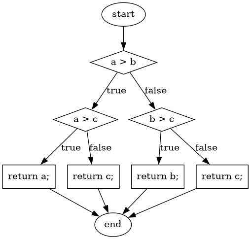
The cyclomatic complexity of a program, represented by its control flow graph, is defined as \$v(G) = E - V + 2P\$, where \$N\$ is the number of nodes, \$E\$ the number of edges and \$P\$ the number of connected components of the underlying undirected graph. In the way we have defined the control flow graph, \$P\$ is always 1. This metric is directly derived from the cyclomatic number or circuit rank of the undirected graph. This property represents the minimum number of edges that has to be removed in order to break all cycles and obtain a spanning tree.
McCabe showed that the computation of the cyclomatic complexity could be simplified as the number of predicate nodes (conditionals) plus one. The method in Listing 12 has a cyclomatic complexity of \$v(G) = 4 = 3 + 1\$, as it has three conditionals: a > b, a > c and b > c. It can be also computed as \$v(G) = 4 = 11 - 9 + 2\$, as it has eleven edges, nine nodes and only one connected component.
McCabe’s cyclomatic complexity is well known and widely used. It is frequently accompanied by a scale. Values below 10 are usually considered as good. However, some caveats of the metrics must be taken into account. First, it was conceived for unstructured programs and some aspects of its original definition are vague. Modern tools implementing the metric work under different assumptions, therefore two different tools may not produce the same result for the same method. Logical conjunctions and disjunctions (&& and || in some programming languages) also produce branches but not all tools include them in their results.
Not always the cyclomatic complexity matches the developer’s idea of what is a complex method. For example, the metric does not consider nested structures. It produces the same value for the two code fragments in Listing 13.
// 1
if (a) {
    if (b) {
        ...
    }
    else {
        ...
    }
}
else {

}

//2
if(a) {
    ...
}
else {

}
if (b) {

}
else {

}
In (42), the author advocates against the use of the metric. Besides showing concrete examples where tools produce different results, he discusses the method in Listing 14. The author explain that this method is fairly easy to understand, yet it has a cyclomatic complexity of 13 while the more complex method in Listing 15 has a cyclomatic complexity of 5.
String getMonthName (int month) {
    switch (month) {
        case 0: return "January";
        case 1: return "February";
        case 2: return "March";
        case 3: return "April";
        case 4: return "May";
        case 5: return "June";
        case 6: return "July";
        case 7: return "August";
        case 8: return "September";
        case 9: return "October";
        case 10: return "November";
        case 11: return "December";
        default:
            throw new IllegalArgumentException();
    }
}int sumOfNonPrimes(int limit) {
int sum = 0;
OUTER: for (int i = 0; i < limit; ++i) {
if (i <= 2) {
continue;
}
for (int j = 2; j < i; ++j) {
if (i % j == 0) {
continue OUTER;
}
}
sum += i;
}
return sum;
}Coupling between objects or class coupling
A class is coupled to another if the former uses a method or a field from the latter. Coupling between classes can not be avoided, it is, in fact, desirable. We create classes as functional units for reuse. At some point, existing classes will be leveraged to create new functionalities. However, coupling has important implications: changing a class will, most of the times, require changing its dependent classes. Therefore, tight coupling between classes harms modularity and makes a software too sensitive to change and harder to maintain (43) (44).
Class coupling or Coupling Between Objects (CBO) of a class is the number of external classes it uses. In Listing 16, Point has CBO of 0. It only depends on double and the metric does not consider primitive types. Line, on the other hand, depends on Point and has a CBO of 1. The metric counts only unique classes. In the example, Line uses Point several times, but it is counted only once.
Point as CB=0 coupling and Line 1.class Point {
private double x, y;
public Point(double x, double y) {
this.x = x;
this.y = y;
}
public double getX() {
return this.x;
}
public double getY() {
return this.y;
}
public double dot(Point p) {
return x*p.x + y*p.y;
}
public Point sub(Point p) {
return new Point(x - p.x, y - p.y);
}
}
class Segment {
private Point a, b;
public class Segment(Point a, Point b) {
this.a = a;
this.b = b;
}
public boolean has(Point p) {
Point pa = p.sub(a);
Point ab = a.sub(b);
double product = pa.dot(ab);
return 0 <= product && product <= ab.dot(ab);
}
}Classes with low CBO values, or loosely coupled are easier to reuse. Classes with large CBO values or tightly coupled should be avoided and refactored. If a tightly coupled class is necessary, then it requires rigorous testing to correctly verify how it interacts with all its dependencies.
Coupling could be measured not only at the class level but also between any modules at all granularity levels (e.g., packages, components…).
The Law of Demeter (LoD) or principle of least knowledge is a guideline aiming to keep classes loosely coupled (46). Its idea is that any unit should only "talk" to "its closest friends" and not to "strangers". In the context of Object-Oriented Programming, it means that a method can only invoke methods from the receiver (this), a parameter, an object instantiated in the method or an attribute of the class. Listing 17 shows examples of a good use and some violations of this principle.
public class Foo {

    public void example(Bar b) {
       C c = b.getC(); (1)

       c.doIt(); (2)

       b.getC().doIt(); (3)

       D d = new D();
       d.doSomethingElse(); (4)
    }
}| 1 | Conforms to LoD |
| 2 | Violates LoD as c was not created inside example |
| 3 | Chaining method invocations does not conform to LoD |
| 4 | Conforms to LoD, as d was created inside the method |
LoD has downsides as well. A strict adherence to its postulates may produce many unnecessary wrapper methods. In Listing 17 the class Bar should had a wrapper method doItInC whose code could be this.getC().doIt() or something alike. This kind of wrapper would be widespread in the code and it could become a challenge for maintenance. On the other hand, fluent APIs encourage the use of method chains, which also tends to improve readability.
Class cohesion
A class in an object-oriented program, or a module in general, is expected to have a responsibility over a single and well defined part of the software’s functionalities. All services/methods of the module/class should be aligned with this responsibility and this responsibility should be entirely encapsulated in the class. This ensures that the module/class is only changed when the requirements concerning the specific responsibility change. Changes to different requirements should not make a single class to change (47) (48). This is known as the The Single Responsibility Principle and it was coined by Robert C. Martin in the late 1990’s. This principle puts the S in the SOLID principles of object-oriented programming.
| The SOLID principles of object-oriented programming are: S: Single Responsibility Principle, O: Open/Closed Principle, L: Liskov’s Substitution Principle, I: Interface Segregation Principle and D: Dependency Inversion Principle. |
If a class violates this principle, then it can probably be divided in two or more classes with different responsibilities. In this case we say that the class lacks cohesion. In a more concrete view, a cohesive class performs different operations on the same set of instance variables (43).
There are several metrics to evaluate cohesion in classes, but most of them are based in the Lack of Cohesion Of Methods (LCOM) (43). This metric is defined as follows:
Let \$C\$ be a class with \$n\$ methods: \$M_1, ..., M_n\$, let \$I_j\$ the set of instance variables used by the method \$M_j\$. Let \$P = { (I_i, I_j) | I_i \cap I_j = \emptyset, i \gt j }\$, that is, the pairs of methods that use disjoint sets of instance variables, and \$Q = { (I_i, I_j) | I_i \cap I_j \ne \emptyset, i \gt j}\$, all pairs of methods using at least one instance variable in common. Then \$\text{LCOM}(C) = |P| - |Q| \text{ if } |P| \gt |Q| \text{ 0} \text{ otherwise}\$.
This means that LCOM is equal to the number of pairs of methods using a disjoint set of instance variables minus the number of pairs of methods using variables in common. If the class has more methods using disjoint sets of instance variables then it is less cohesive. A class is cohesive if its methods use the same variables to compute different things. Low values of LCOM are preferred.
Table 2 shows the set of all instance variables used by each method declared in the Point class shown in Listing 16. Constructors are not used to compute this metric, as their role is to initialize the variables and they virtually access all of them. In this particular example, all methods use the instance variables directly. However, a method could use an instance variable indirectly by invoking other methods. In that case, the variables are also said to be used by the initial method. For example, any new method invoking getX in Point would also use variable x.
| Method | Instance variables |
|---|---|
|
{ |
|
{ |
|
{ |
|
{ |
Table 3 shows the instance variables used un common for all pairs of methods declared in Point. Only getX and getY do not use any variable in common.
getX |
getY |
dot |
|
|---|---|---|---|
|
{ |
{ |
{ |
|
{ |
{ |
|
|
\$\emptyset\$ |
||
Given that we obtain: \$ | P | = | \{ (I_\text{getX},I_\text{getY}) \} | = 1 \$ and: \$ | Q | = | \{ (I_\text{getX},I_\text{sub}), (I_\text{getX},I_\text{dot}), (I_\text{getY},I_\text{sub}), (I_\text{getY},I_\text{dot}), (I_\text{dot},I_\text{sub}) \} | = 4\$ producing: \$ \text{LCOM}(C) = 0 \$ as \$ | P | \lt | Q | \$. Which means that the Point class is cohesive, its carries the responsibility to represent the concept of a two-dimensional point. Only a change in the requirements of this representation will make this class change.
Lack of cohesion implies that a class violates the principle of single functionality and could be split in two different classes. Listing 18 shows the Group class. The only two methods in this class use a disjoint set of fields. compareTo uses weight while draw uses color and name. Computing the metric we get: \$\text{LCOM}(C = |P| - |Q| = 1 - 0 = 1\$.
compareTo and weight could be separated from the rest.class Group {
private int weight;
private String name;
private Color color;
public Group(String name, Color color, int weight) {
this.name = name;
this.color = color;
this.weight = weight;
}
public int compareTo(Group other) {
return weight - other.weight;
}
public void draw() {
Screen.rectangle(color, name);
}
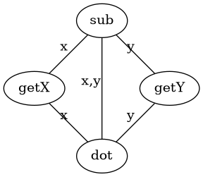
}Tight Class Cohesion (TCC) and Loose Class Cohesion (LCC) are other two well known and used metrics to evaluate the cohesion of a class (49). Both these metrics start by creating a graph from the class. The graph is constructed as follows: Given a class C, each method m declared in the class becomes a node. Given any two methods m and n declared in C we add an edge between m and n if and only if, m and n use at least one instance variable in common. Going back to the definition of LCOM, we add an edge between m and n if \$I_{m,n} \ne \emptyset\$. TCC is defined as the ratio of directly connected pairs of node in the graph to the number or all pairs of nodes. On its side, LCC is the number of pairs of connected (directly or indirectly) nodes to all pairs of node. As before, constructors are not used.
Figure 8 shows the graph that results from the class Point. In this example there are 5 edges or direct connections, and, as there are 4 nodes, then there are 6 node or methods pairs in total. Therefore \$\text{TCC = 5/6 = 0.83\$. On the other hand, all nodes are connected and \$\text{LCC} = 6/6 = 1\$.
If we do the same for the Group class, we obtain a graph where all nodes are disconnected and both LCC and TCC are 0.
In object-oriented programs a class may inherit methods and instance variables from its base classes. In those cases, computing the cohesion of a subclass may: include only inherited methods, only inherited fields, or both. The original definitions of TCC and LCC are open with respect of inherited members. Users of the metrics should decide whether to include them or not (49).
2.2. Static analysis
Enforcing coding guidelines, detecting code smells and computing code metrics, can and should be automated. All these goals can be achieved by inspecting the code without executing the program. This is known as static analysis. Any form of static analysis takes as input the code of a program. It may be a high level code, such as Python, or Java, or it could also target compiled code as the JVM bytecode. The static inspection of code also enables the early detection of problems like cyclic dependencies, potential null pointer exceptions, buffer overflows. Since it does not require the execution of the program, static analysis is, in most cases, very efficient in terms of computation time.
There are plenty of tools available that can perform many types of static analysis. Some of them are highly configurable to, for example, select the coding guidelines a team wants to enforce. Many of these tools are also extensible and may allow the incorporation of new metrics, code smell definitions and other unforeseen functionalities. There are also libraries that make it easy to implement custom static analysis tools. This section presents some of these libraries and tools for Java.
2.2.1. Implementing a static analysis
Most code analyses start with the two same initial phases of a compiler: the lexicographic and syntactic analyses.
Given a source code, say in Java as the one in Listing 19, a lexicographical analyzer, lexer, or scanner, groups together sequences of characters. These sequences are usually associated with a type and are called tokens. The lexer produces as output a sequence of tokens.
class A {

    public void method() {
        System.out.println("Hello");
    }
}
Listing 20 shows the first tokens produced by a lexer for the code in Listing 19. A lexer also removes characters that are not needed for subsequent phases like white spaces and comments.
("class", CLASS_KEYWORD)
("A", IDENTIFIER)
("{", "OPEN_BRACE")
("public", PUBLIC_KEYWORD)
("void", VOID_KEYWORD)
("method", IDENTIFIER)
The sequence of tokens is used as input for the syntactic analysis where a parser checks that the order of the tokens is correct with respect to a formal specification or grammar and builds an Abstract Syntax Tree (AST). An AST is a hierarchical representation of the source code. The nodes represent the elements in the code in a way that, for example, nodes representing classes have children representing methods and fields, and nodes representing methods contain nodes representing instructions. The AST does not contain purely syntactical elements such as semicolons or braces. Figure 9 shows a simplified version of an AST for the code in Listing 19.
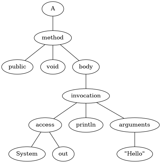
Most static analyses are implemented by tracing the AST and most implementations are based on the visitor pattern. The visitor pattern abstracts the operations to be performed over an object structure (50). Each operation is implemented as a visitor. The structure is traversed and each visitor is selected according to the elements of the structure that is being visited. In the case of a static analysis over an AST, each visitor could be a class or a method, designed to operate over a specific type of node, for example, a class will be handled by a class visitor. The static analysis is then carried by the joint actions of these visitors.
There are libraries that facilitate the implementation of static analyses by accomplishing the construction of the AST and even providing abstractions to implement the visitor pattern. For Java sources two of the most famous are Spoon and JavaParser. There are other libraries that offer similar functionalities but targeting compiled code. One most famous JVM bytecode analysis tool is ASM.
Using JavaParser
This section explains how to implement a simple static analysis tool using JavaParser. As a library, JavaParser provides a hierarchy of classes to represent ASTs for Java programs and implementations of the visitor pattern to help analyze and transform those ASTs.
Figure 10 shows a selection of classes representing AST nodes. Node is the base class of the hierarchy. The instances of ClassOrInterfaceDeclaration represent declarations of classes and interfaces in the program. These nodes contain information about the type parameters, base class and interfaces implemented in the corresponding declaration. ClassOrInterfaceDeclaration inherits from the more general TypeDeclaration, which contains, among other properties, a name. TypeDeclaration inherits from BodyDeclaration which is also the base class for all elements that could be included in the body of a type declaration. Expression is the super class of all abstractions of expressions as it is the case for MethodCallExpr and FieldAccessExpr. Both these classes contain information about the scope or receiver of the method call or the field access, as well as the name of the method or the field. MethodCallExpr also provides information about the arguments. On its side,Statement is the base class for all types representing statements in the program, as it is the case of the IfSmt. This last class has an Expression representing the condition and two Statement instances for the then and else branches of the conditional statement.
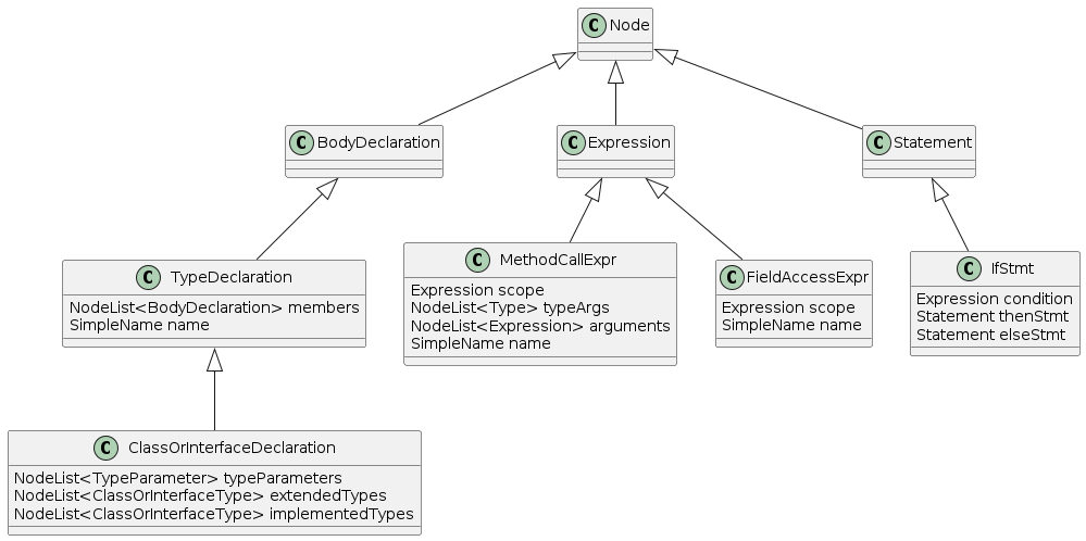
The visitor pattern is implemented in JavaParser by the interfaces VoidVisitor (Listing 21) and GenericVisitor (Listing 22). Both interfaces are very similar. They both contain visit methods for all concrete classes representing AST nodes. In the former interface these methods are void while the latter allows to return a value. This is the only difference. All visit overloads also accept an arg parameter to share information among nodes in the traversal of the AST.
VoidVisitor class in JavaParser.public interface VoidVisitor<A> {
...
void visit(ClassOrInterfaceDeclaration n, A arg);
void visit(IfStmt n, A arg);
void visit(MethodCallExpr n, A arg);
void visit(FieldAccessExpr n, A arg);
...
}GenericVisitor class in JavaParser.public interface GenericVisitor<R, A> {
...
R visit(ClassOrInterfaceDeclaration n, A arg);
R visit(IfStmt n, A arg);
R visit(MethodCallExpr n, A arg);
R visit(FieldAccessExpr n, A arg);
...
}There is no need to directly implement these two interfaces. The library also provides some default implementations to ease reuse. For example, VoidVisitorAdapter and GenericVisitorAdapter implement the visitor interfaces and perform a depth-first traversal of the AST. A new visitor could extend one of these adapter classes and just redefine the visit overloads it actually needs and not all of them. ModifierVisitor enables a similar reuse, but specialized on the use case where the AST should be modified. Listing 23 shows a fragment of the code of this class implementing the visit method overload for IfStmt.
ModifierVisitor class in JavaParser.public class ModifierVisitor<A> implements GenericVisitor<Visitable, A> {
@Override
public Visitable visit(final IfStmt n, final A arg) {
Expression condition = (Expression) n.getCondition().accept(this, arg); (1)
Statement elseStmt = n.getElseStmt().map(s -> (Statement) s.accept(this, arg)).orElse(null); (2)
Statement thenStmt = (Statement) n.getThenStmt().accept(this, arg); (3)
Comment comment = n.getComment().map(s -> (Comment) s.accept(this, arg)).orElse(null); (4)
if (condition == null || thenStmt == null) (5)
return null;
n.setCondition(condition); (6)
n.setElseStmt(elseStmt);
n.setThenStmt(thenStmt);
n.setComment(comment);
return n;
}
}| 1 | The condition expression is visited and the result is stored in condition. |
| 2 | The else part is visited and the result is stored in elseStmt. |
| 3 | The then part is visited and the result is stored in thenStmt. |
| 4 | If there is any comment associated to the statement, it is also visited. |
| 5 | In the case there is no valid result for the mandatories condition and then part, the result is null. |
| 6 | Otherwise the node is updated with the result from visiting the children elements and the method returns its reference. |
With the help of JavaParser we will implement a small tool to enforce a coding convention. In Java, and many other languages, it is optional to use braces ({}) in loops and conditionals if the body contains only one statement. For example, it is not easy to see that the else belongs to the inner conditional statement in Listing 24. Also it is easy to missplace code when not using the braces.
class A {
    public void m() {
        boolean a = true, b = false;
        if (a) if(b) System.out.println("one"); else System.out.println("two");
    }
}
Using ModifierVisitor as base, we will implement a visitor that modifies the AST so that the then and else parts of all conditional statements are enclosed in braces, that is, the statements must be contained in a block. The implementation of this custom visitor is shown in Listing 25. The BlockEnforcer traverses the AST and modifies only IfStmt nodes. It ensures that each then and else parts are instances of BlockStmt. Notice the use of Void as a type parameter for the implementation as no extra information will be passed between nodes.
public class BlockEnforcer extends ModifierVisitor<Void> {

    @Override
    public Visitable visit(IfStmt n, Void arg) {
        IfStmt result = (IfStmt) super.visit(n, arg); (1)
        if (result == null) { (2)
            return null;
        }
        result.setThenStmt(enforceBlockOn(result.getThenStmt())); (3)
        result.getElseStmt().ifPresent(statement ->
                result.setElseStmt(enforceBlockOn(statement))); (4)
        return result;
    }

    public Statement enforceBlockOn(Statement stmt) { (5)
        if (stmt.isBlockStmt()) { (6)
            return stmt;
        }
        BlockStmt block = new BlockStmt(); (7)
        block.addStatement(stmt);
        return block;
    }
}| 1 | Perform the original traversal and propagate the analysis to the children elements. |
| 2 | Return null if the result from the children is also null. |
| 3 | Enforce a block in the then part. |
| 4 | Enforce a block in the else part if present. |
| 5 | enforceBlockOn takes a statement and returns a block. |
| 6 | Do nothing if the initial statement is already a block. |
| 7 | Otherwise, create a new BlockStmt containing the initial statement. |
Listing 26 shows how to use BlockEnforcer to analyze a single Java file. The first step is to obtain an instance of CompilationUnit. A compilation unit in Java is a file that optionally declares a package and contains an arbitrary number of imports and type declarations. StaticJavaParser provides shortcut methods to get such objects from common String, InputStream, Reader and File inputs. Then the visitor is applied through the accept method. This snippet prints on the screen the result of the analysis by invoking the toString method of CompilationUnit. The result cane be also saved to a file or we can even rewrite the original source code.
BlockEnforcer to analyze a single Java file.CompilationUnit unit = StaticJavaParser.parse(input); (1)
unit.accept(new BlockEnforcer(), null); (2)
System.out.println(unit.toString()); (3)| 1 | Obtain a CompilationUnit instace. input could be a String, Reader, InputStream or File. |
| 2 | The compilation unit is visited to start the analysis. |
| 3 | The result is printed to the screen. |
When given the code in Listing 24, Listing 26 produces Listing 27 as result.
class A {

    public m() {
        boolean a = true;
        boolean b = false;
        if (a) {
            if (b) {
                System.out.println("one");
            } else {
                System.out.println("two");
            }
        }
    }
}
Of course, JavaParser also includes functionalities to analyze a full Java project and more. Further information can be found in the project’s website.
2.3. Tools for static analysis
There are plenty of static analysis tools for all languages and frameworks. Compilers are the first of such tools we use. They rely on static analysis to check the syntactic and semantic validity of the program. Compilers may also detect unreachable code, unused variables and potential conversion errors.
Other tools, often called linters, help improve the quality of the program by detecting code smells, proposing code improvements and enforcing coding guidelines. In most cases they are highly customizable and extensible so each team, project or company can adapt the linter’s functionalities to their own practices and goals. The term linter comes from lint a tool conceived to analyze portability issues for C programs back in the 70’s.
For Java, the most popular alternatives are:
-
Error Prone: Detects common bug patterns and proposes potential fixes. For example, the tool is able to detect wrong printf-style formats used in the code.
-
SpotBugs: Also finds known bug patterns and bad practices, but targets the compiled bytecode instead of the source code. For example, it can propose use a more efficient equivalent method such as use
Integer.valueOfinstead ofnew Integer. -
checkstyle: Detects coding guideline violations. For example, it checks that a class with only one private constructor is declared as final, as it can not be extended anyways.
-
PMD: A cross-language static analysis tool able to detect code smells, compute code metrics, and detect guideline violations. For example, it computes the Cyclomatic Complexity of a method and the Tight Class Cohesion (TCC) as seen before. It can also recommend, for example, when to replace a
forby aforeach.
All the tools mentioned above are able to detect several hundreds of know bug patterns, code smells and bad practices. They are also configurable and extensible via plugins.
2.3.1. Using and extending PMD
PMD is one of the most complete alternatives available. It uses a huge and modifiable set of rule definitions to detect code patterns representing code smells and potential bugs. It can be extended with custom rules and metrics. This section shows how to use PMD and how to extend it.
The tool can be freely downloaded from its website as a zip file. This file contains the PMD program itself and the files corresponding to the rule definitions. It can be used from the command line as follows:
<path-to-pmd-folder>/bin/run.sh pmd -d <path-to-java-file> -f text -R <path-to-rule-definition>The line above runs PMD over a single Java file using a single rule definition file and outputs the result to the console in plain text.
The PMD documentation contains a comprehensive list of all rules PMD includes for Java. These rules are sorted into categories according to their nature. For example, the Design category contains rules that discover design issues. One of the rules inside this category is AbstractClassWithoutAnyMethod. As it name indicates, it finds and signals abstract classes without any declared method. The rationale behind this rule is that the abstract modifier has been added so no instance of this class can be created. In that case, it is better to have a private constructor.
Let the code in Listing 28 be the content of SillyClass.java.
public abstract class SillyClass {
    String field;
}
The rule can be invoked as follows:
<path-to-pmd-folder>/bin/run.sh pmd -d SillyClass.java -f text -R category/java/design.xml/AbstractClassWithoutAnyMethodSee that category/java/design.xml is an internal PMD route to the design.xml which contains the definition of all rules targeting design issues in Java.
In the Error Prone category, PMD includes the CloseResource rule. This rule finds code where resources are not properly closed. As an example in Listing 29 the Bar class does not close the Connection resource. PMD signals an error when passed this code to the CloseResource rule. The solution is to call c.close() in a finally block.
Connection is not closed.public class Bar {
public void foo() {
Connection c = pool.getConnection();
try {
// do stuff
} catch (SQLException ex) {
// handle exception
}
}
}If the CloseResource rule is used in the code from Listing 30, PMD will report an error even when the connection is effectively closed in another method. The tool fails to see that the resource is closed in bar as the rule matching does not go beyond the code of foo. PMD does not analyze how methods invoke each other, probably to keep the analysis and rule matching simple and scalable.
We can consider tools like PMD as an algorithm that classifies a piece of code into issue and not issue. In this sense, Listing 30 is an example of a false positive, that is, an error reported by PMD in a situation where the problem does not occur.
Connection is closed in another method but PMD still produces an error.public class Bar {
public void foo() {
Connection c = pool.getConnection();
try {
// do stuff
} catch (SQLException ex) {
// handle exception
} finally {
bar(c);
}
}
public void bar(Connection c) {
c.close();
}
}The CloseResource rule signals no error when given the code in Listing 31 as input. However, in this code it is clear that, if an exception is thrown, the resource will not be closed. This is an example of a false negative: no issue was signaled by the tool, when there is actually one.
public class Stream {
    BufferedReader reader;

    public void readData()  {
        try {
            String line = reader.readLine();
            while (line != null) {
                System.out.println(parseLine(line));
                line = reader.readLine();
            }
            reader.close(); (1)
        } catch (Exception e) {
            e.printStackTrace();
        }
    }
}| 1 | If the code above throws an exception the resource is never closed. |
PMD searches for patterns in the source code and these patterns may not include all cases, as seen in the two examples above. This is a limitation of static analysis in general. The code is not executed, therefore no dynamic behavior is considered, as in the case of Listing 31 where the issue is influenced by the input of the user.
It is possible to extend PMD with new rule and metric definitions. This is useful to accommodate PMD to custom requirements. For example, a team can define their own set of rules to reflect their best practices when using third party library or framework like Hibernate or Spring.
PMD provides a complete API to implement custom rules and metrics. As with the libraries discussed before, this API relies on a visitor pattern over the AST of the source code. Defining new metrics or rules this way is very similar to what can be done with JavaParser.
However, there is another simpler alternative that does not require to program a new rule. As long as the rule requires only to query the AST looking for patterns, it could be written using XPath.
XPath stands for XML Path Language. It is a language used to express queries selecting nodes in an XML document based on their relationship with their ancestors, descendants and the value of their attributes. An XML document is, in fact, a tree. Therefore it does not require any special adaptation to use XPath and select nodes from an AST. PMD allows to define rules in this way.
A rule defined using XPath consists in a selection query. If the query finds a match, then an error is reported. Retaking the example of BlockEnforcer to signal that a conditional statement must use braces, the query would be:
//IfStatement/Statement[not(./Block)]//IfStatement/Statement matches the direct Statement children of any IfStatement node, this matches the then and else children nodes. not(./Block) matches no direct descendant of type Block. So the entire expression matches conditionals whose then and else nodes do not have a direct Block descendant.
The rule must be specified in an XMl file. Those files may contain definitions of more than one rule. The full code for this example is shown in Listing 32.
<?xml version="1.0"?>

<ruleset name="Custom Rules"
    xmlns="http://pmd.sourceforge.net/ruleset/2.0.0"
    xmlns:xsi="http://www.w3.org/2001/XMLSchema-instance"
    xsi:schemaLocation="http://pmd.sourceforge.net/ruleset/2.0.0 http://pmd.sourceforge.net/ruleset_2_0_0.xsd">
    <description>
        Custom rules
    </description>
    <rule
    name="MandatoryBracesOnIf"
    language="java"
    message="Then and else parts of a conditional statement must be enclosed by braces"
    class="net.sourceforge.pmd.lang.rule.XPathRule">
    <description>
        Then and else parts not enclosed by braces in a conditional statement
        may harm readability and facilitate the introduction of bugs.
    </description>
    <priority>3</priority>
    <properties>
        <property name="xpath">
        <value><![CDATA[
            //IfStatement/Statement[not(./Block)]
        ]]></value>
        </property>
    </properties>
    </rule>
</ruleset>
2.4. Static analysis in the development process
There are several ways to include linters and other static analysis tools in the development process. Most Integrated Development Environments (IDE) such as Eclipse or IntelliJ IDEA and code editors like Atom or Visual Studio Code, support them and even have them preinstalled out-of-the-box. IDE integration allows programmers to obtain instant feedback while coding.
Such tools can also be integrated in the compiling or building process. Utilities like Maven or Gradle permit the addition of custom build actions through plugins. Static analysis tools could be incorporated to the process as plugins and even make the build fail under certain conditions. In fact, there is already a PMD Maven plugin. With this plugin it is possible to generate a full report of issues discovered by PMD in the code of a project. This report could be exported in human readable formats like HTML or files adapted for automation like CSV and XML. The plugin can be configured with a selection of rules and provide means to make the build fail if there are issues with a given level of severity. As with any Maven plugin, this one can be attached to a build step so, for example, it is launched every time the compilation process starts without having to invoke the plugin directly.
Most projects are not developed by a single person. Projects are regularly built by a team of developers that may not even use the same development environment and may have different coding practices. Static analysis tools become then great allies to find potential issues and to keep the code understandable. In those cases, these tools may be better used with the help of Continuous Integration (CI) servers. These servers, like Jenkins or Travis monitor the code repositories and execute the analysis tools on every commit or for pull requests (Figure 11). In this way all new additions to the project are automatically inspected. Integration could even go further and automatically report all the issues that were found in the new code. Major source hosting services provide their own CI solutions like Github Actions and Gitlab CI that are a good fit for this kind of integration scenario.
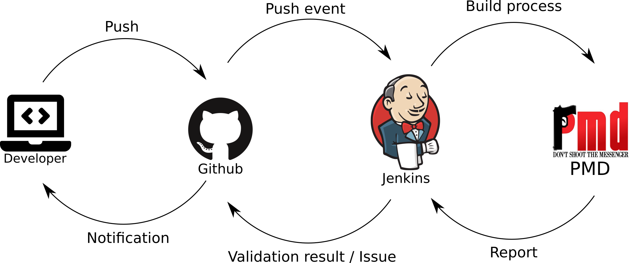
Nowadays it is a common practice in companies and open source projects to watch the quality of their code through manual inspection. These inspections are known as code reviews. In companies like Google, for example, every code change should be manually reviewed (51).
A typical code review may involve people in 4 main roles: a moderator, the programmer responsible for the code under inspection, a system designed and the code inspector. The involvement of different roles helps in having different points of view and a more global system-wide perspective. In the review, the system designer and the inspector use their expertise to get a list of potential issues in the code being inspected. These issues are discussed with the programmer who shall fix those that represent actual problems after the review. The process could be implemented as a formal meeting or deferred using a dedicated platform and even echanging direct messages.
A code review is successful only if it is carried with very clear goals. For example, reviewing a change in the code may involve answering the following questions:
-
Is the code clear enough?
-
Could the development of the program be continued by someone other than the programmer?
-
Are there redundancies in the code?
-
Are there asymmetries like missing cases in the input validation?
Static analysis tools help making code reviews more systematic by finding potential issues that might be missed by the inspector. CI integration is specially helpful for this kind of process.
There are tools that implement and automate code review processes. For example Github includes a review workflow for pull requests. The code in the pull request could be annotated and verified either manually or using automated tools. The platform facilitates the exchange between the developer that originated the pull request and the inspector.
SonarQube has become one of the major players in this area. The tool integrates with most used CI/CD and source hosting services. It supports 27 different programming languages and evaluates the quality of the code using a comprehensive set of metrics and vulnerabilities and smell detectors. The platform also helps in the organization of the project by automatically assigning the issues it finds to the developers that made the change.
Static analysis tools help assuring the quality of the code. They can efficiently spot potential issues and can be easily integrated in the development process at different levels. However, these tools do not run the code which makes them specially prone to false positives. They should be complemented with other tools that observe the execution of the program under different conditions, that is, dynamic analysis tools and testing.
3. Software Testing
According to Ammann and Offutt [ammann2016introduction] Software Testing is the process of evaluating a software by observing its execution to reveal the presence of faults. Or, as Meyer says in his principles (23) "`to test a program is to try to make it fail`". Per this definition, testing (aka. dynamic testing) is a form of dynamic analysis: it requires the execution of the program or system under test.
Testing is achieved through the design and application of test cases. In broad terms, a test case is a set of steps and values that must provide the required input and set the program in the desired state by triggering specific behaviors. It then, must check the output of the program against expected results. Often, the output of the test case execution is validated with an oracle, i.e. a predicate to tell whether the execution was successful or not. A test case may optionally include prefix values which are inputs necessary to get the system ready for the input and postfix values which are inputs needed to clean the environment after the execution of the test. Test cases may be functional, if they check that a functionality is correct, or non-functional if it is directed to evaluate properties like performance, security or even energy consumption. If a test case executes normally it is said to pass otherwise, if the output is not correct, we say that there is a test failure and that the test fails.
A test case exercises the system in one specific scenario. So, only one test case is not enough to correctly verify the system. Therefore we always need to create a set of multiple test cases. This set is usually called test suite.
3.1. Levels of testing
- Unit Testing
-
It is the lowest level of testing and targets the code units of the program: procedures, functions or methods. The goal is to assess the implementation of the software. For example, a unit test for a function that computes the factorial of a given number, would call the function with an input, say 5 and then check that the result is 120.
- Module Testing
-
Units are often grouped in modules that could be classes, packages or files. This level of testing verifies each module in isolation and evaluates how the component units interact with each other. For example, a test for a
Stackclass may create an instance of the class, push an element onto the stack, pop it out and finally check that the stack is empty.
| In Object-Oriented Programming a class is at the same time a unit and a module. Therefore the distinction between unit tests and module tests is not clear within this context. In fact, for most testers and developers both types of testing are known as unit testing and it will be also the case for the rest of this text. |
- Integration Testing
-
The goal of this level of testing is to assess the interaction between modules and verify that they are communicating correctly. Integration tests assume that modules work correctly. Modules should be verified by the previous testing levels. As an example, an integration test for an online store may check the interaction between the shopping cart module and the payment gateway by creating and validating an order, or it could also verify that data access abstractions communicate correctly with the database by creating the right queries and interpreting the results in the right way.
- System Testing
-
The goal of this level is to check whether the assembled system meets the specifications. Thus, it assumes that all subsystems work correctly, which is the task of the previous testing levels. System tests execute the system as a whole from beginning to end, that is why they are sometimes also referred as end-to-end tests. An example of such tests in the context of an online store could verify that: a user can log in with the right credentials, she can create a shopping cart with a selection of products, she can validate the order, she receives an email with the invoice and then she is able to log out. Testing done from the graphical user interface is also a form of system testing.
- Acceptance Testing
-
This level checks that the finished product meets the needs of the users, that is, if the system does what users want. These tests should be elaborated from the user’s perspective and may be used to evaluate the requirements. Like system tests, these also verify the product from beginning to end.
| There might be other, even finer-grained, classifications for tests and they all tend to be blurred and even ambiguous. Classifying one test case as unit, module, integration or system is not crucial. The most important message here is that testing should be carried at different levels, for each unit, whatever they may be, then how these units interact and then how the entire system behaves. |
Each level of testing has its own level of complexity. Unit tests tend to be easier to define and faster to execute. System tests are more complex and slower. Inputs for unit tests may not be completely realistic compared to the inputs that shall appear in production and they are not generally able to find faults arising from the interaction of modules. System tests tend to be more realistic. On the other hand, finding an implementation fault from a system test may be even impractical.
Automating the execution of tests at all levels is key for modern software development practices. Manual tests are tedious, take a lot of time and are prone to errors. Automated test execution allows having more tests and therefore more scenarios are explored. As Meyer explains in his fourth principle,(23) it is not feasible to manually check the output of hundreds of tests. Automated tests help producing a faster, almost immediate feedback during development on whether certain types of faults are being inserted. In this way they enable efficient CI/CD processes which facilitate the integration of the work of development teams. Automated tests help also preventing regressions that is, the reinsertion of an already solved fault. This is specially true if we adhere to Meyer’s third principle “Any failed execution must yield a test case, to remain a permanent part of the project’s test suite” (23).
The accepted practice nowadays is to have most tests automated, while keeping only a small amount of manual tests, mainly as acceptance tests. Most organizations have a large number of unit tests, which are easier to write, faster to execute and easier to understand. Organizations tend to have less system tests which are more complex, expensive and harder to maintain. This is reflected on what is known as the testing pyramid Figure 12.
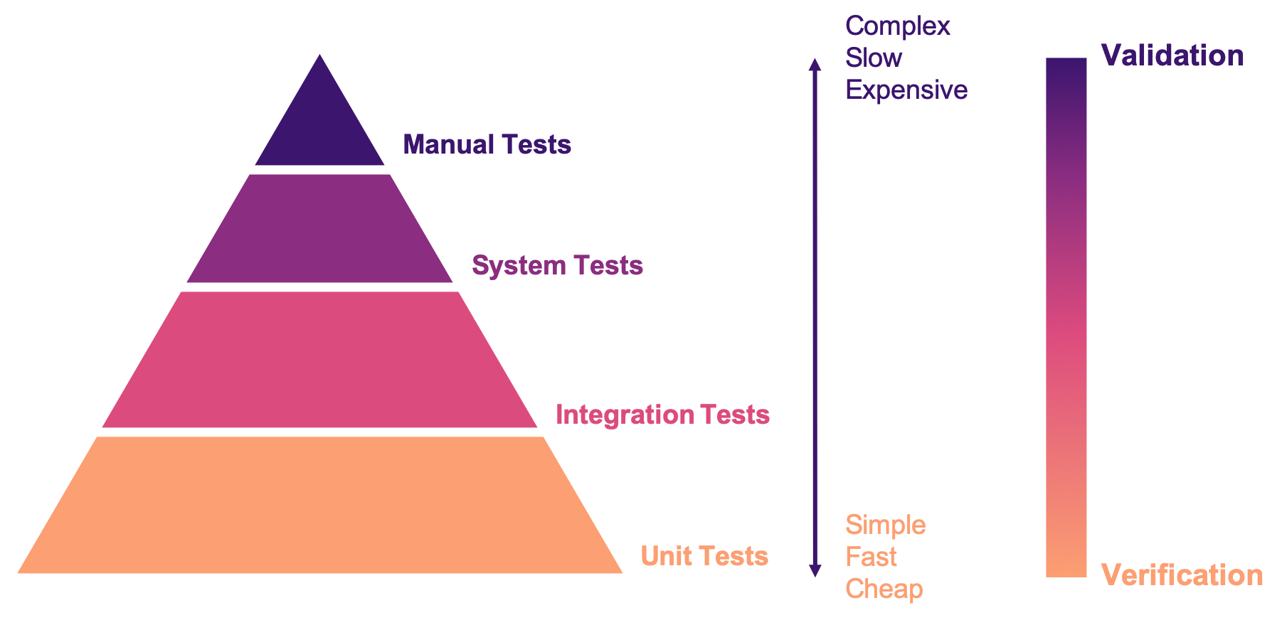
So, as we move up in the pyramid from unit tests, which directly assess the implementation of the system, to acceptance tests which check the compliance of the system with the users' needs, we move from the area of verification to the area of validation.
3.2. Test automation frameworks: JUnit
Test automation allows having more tests to explore more execution scenarios, provides a faster feedback and facilitates integration processes. It is achieved with the help of test automation frameworks or testing frameworks.
A testing framework is a set of tools and libraries providing mechanisms to define or specify test cases and execute them. One of the most famous alternatives at the moment is JUnit, initially developed by Kent Beck in 1997. JUnit has become a sort of de-facto standard for Java projects and has inspired the creation of similar frameworks for other languages and platforms which are informally called as the xUnit family. Despite having “unit” in the name and being widely used for unit testing, the framework can be use to implement all sort of automated tests.
| At the moment of writing this material the latest stable version of JUnit is 5.7.1. This version will be used for all code examples. |
Suppose we have the BoundedStack class, shown in Listing 33, that implements a LIFO (Last In First Out) data structure with a fixed capacity. The class has a void method push to insert an element onto the stack, and pop that removes the element on top of the stack and returns it.
BoundedStack class represents a LIFO data structure with maximum capacity.public class BoundedStack {
private int[] elements;
private int count;
public BoundedStack(int capacity) {
elements = new int[capacity];
count = 0;
}
public void push(int item) {
if(count == elements.length) {
throw new IllegalStateException();
}
elements[count] = item;
count = count + 1;
}
public int pop() {
if(count == 0) {
throw new NoSuchElementException();
}
count = count - 1;
return elements[count];
}
public int size() {
return count;
}
public int capacity() {
return elements.length;
}
}A typical unit test for this class written with the help of JUnit would look like the code shown in Listing 34.
class BoundedStackTest {
    @Test
    public void testPushPop() {
        int original = 1;
        BoundedStack stack = new BoundedStack(10);
        stack.push(original);
        int onTop = stack.pop();
        assertEquals(original, onTop, "Element on top of the stack should be " + original);
    }
}
Test cases in JUnit are implemented inside test classes. These classes declare test methods which contain the main code for the test cases. These test methods are identified with the @Test annotation. In Listing 34 the first four lines of testPushPop provide the input values of the test case and set the instance of BoundedStack in the required state: an element has been pushed and then popped from the stack.
The last line uses an oracle to verify that the element obtained from the stack was the same that was pushed in the first place. This type of oracle is known as an assertion. It evaluates a given condition and if the condition is false an AssertionError is thrown. It also includes a message to use as output in the case the assertion fails. In the absence of any assertion in the code, JUnit tests have an implicit oracle that checks if unexpected errors occur, that is, if an unexpected exception is thrown.
JUnit provides a set of utility methods implementing different assertions such as: assetEquals that checks if two given objects are equal and it is used in the example, assertNotEqual, the contrary, assertNull which verifies if a given value is null, assertSame to verify if two objects are the same and many more.
In some scenarios, a test case should verify whether an operation with the wrong input signals the right error. Listing 35 shows how to achieve this. The test verifies that invoking pop in an empty Stack should throw an IllegalStateException.
@Test
public void testErrorPopEmptyStack() {
    assertThrows(NoSuchElementException.class, () -> {
        new BoundedStack(1).pop();
    });
}
While the assertions included in JUnit cover a wide spectrum of scenarios, libraries like Hamcrest and AssertJ help creating more expressive and higher level assertions.
A test case in JUnit could be more than a single test method, it may include other methods supporting the test execution. For example, methods annotated with @BeforeEach and @AfterEach will be executed before and after each identified test cases in the same test class respectively. These are helpful to set prefix and postfix test inputs.
JUnit includes many additional functionalities to facilitate the creation of tests, such as parameterized tests, special oracles to verify the performance of the code and even the dynamic creation of tests.
It is important to add information that helps identifying the fault in the event of a test failure. In JUnit, and any other testing framework, a common practice to try to achieve this is to use descriptive names for test methods and set detailed messages for assertions. However, there are many other characteristics that good test cases must have in practice.
3.3. Best practices and antipatterns in testing
Automated test cases are code, test code, and like their counter part, the application code, they should be maintained and we should care about their quality. Poorly written test cases bring no value to the development process. They negatively impact the fault detection capabilities of a test suite. They are also hard to understand and hard to leverage to correctly identify faults.
As summarized in (54) automated test cases should be concise and clear: brief, yet comprehensive and easy to understand, self-checking: they should report results without human intervention, repeatable, robust and independent: it should be possible to run them consecutive times without human intervention and they should always produce the same results whether their are run in isolation or with other tests. Tests should also be efficient: they should run in a reasonable amount of time and should be maintainable: that is, they must be easy to modify and extend even when the system under test changes. Also, with respect to the application and the requirements, tests must be sufficient so all requirements of the system are verified, necessary so that everything inside each test contributes to the specification of the desired behavior, with no redundancy and unneeded artifacts, each test should be specific so tests failures point to the specific fault and the broken functionality, and traceable so that it can be easily mapped to the parts of the application code it verifies and the part of the specification it has been derived from.
3.3.1. Test smells
Along the years, the testing community has identified bad practices, smells that deviate from the principles mentioned above and have a negative impact in the quality of tests. Garousi and Küçük (53) reviewed the scientific and industry literature on the subject and were able to identify 179 different test smells. It is important to notice that test smells are not bugs but affect the tests by lowering their efficiency, maintainability, readability, comprehension and their ability to find faults. This section presents and exemplifies some of these test smells.
- Manual intervention
-
Happens when the person running a test case must do something manually before the test is run, during the execution of the test or she should manually verify the results. This practice undermines test automation.
- Testing Happy Path only
-
These tests verify only the common scenario and never check boundaries or input values that should result in exceptions. Most of the time developers write code with the happy path / normal situation in mind and it is most likely that this scenario will work. Therefore, testing only the happy path have lower chances to catch a bug. The test case in Listing 34 tests only the most expected scenario or happy path. We need to add test cases like Listing 35 where we explore extreme scenarios like a pop on an empty stack or when a null element is pushed, or if there is a point at which we can push no more elements to the stack.
- Test logic in production code
-
The application code deployed in production contains logic that should be exercised only during test execution. This logic is there only to support testing, for example, to help tests gain access to the internal state of the application. It also may happen that part of the production logic can not be executed in testing. This makes the system behaves differently in production and testing. An example is shown in Listing 36.
...
if (System.getProperty("env", "prod").equals("test")) {
    return new User('Jane Doe', 'janedoe@example.com'); (1)
}
else {
    User user = new User(Request.getParam(login), Request.getParam(name));
    validateUser(user);
    return user;
}
...| 1 | This line makes the code return a wired values to use in production. |
Another example of this type of smell is when a class does not require an implementation of equals and we do need it just for testing purposes. This is known as equality pollution. The application code is filled with unnecessary equals methods, whose logic may actually go against the requirements.
In general, all forms of this test smell make the application code more complex and introduces maintainability issues.
A way to solve this smell, is to use dependency injection. The code that has to work differently in production and tests can be moved onto a dependency that can be exchanged without affecting the application logic. In case of equality pollution we could use an equality comparer, that is, a class that checks if two objects are equals per our needs.
- Eager test
-
Also known as Test It All or Split Personality. It is a single test that verifies too many functionalities. Listing 37 shows an example of this test smell. When such a test fails, it is hard to tell which code produced the failure. The solution is to separate all verifications into different test cases.
@Test
public void testFlightMileage_asKm2() throws Exception {
    // setup fixture
    // exercise contructor
    Flight newFlight = new Flight(validFlightNumber);
    // verify constructed object
    assertEquals(validFlightNumber, newFlight.number);
    assertEquals("", newFlight.airlineCode);
    assertNull(newFlight.airline);
    // setup mileage
    newFlight.setMileage(1122);
    // exercise mileage translater
    int actualKilometres = newFlight.getMileageAsKm();
    // verify results
    int expectedKilometres = 1810;
    assertEquals( expectedKilometres, actualKilometres);
    // now try it with a canceled flight:
    newFlight.cancel();
    try {
        newFlight.getMileageAsKm();
        fail("Expected exception");
    } catch (InvalidRequestException e) {
        assertEquals( "Cannot get cancelled flight mileage", e.getMessage());
    }
}- Assertion roulette
-
Appears when it is hard to tell which of the many assertions of a test method produced the test failure. This makes harder to diagnose the actual fault. Eager tests tend to also produce assertion roulettes as can be seen in Listing 37. This smell also occurs when assertions do not have any message, as seen in Listing 38. To solve this smell we should refactor the test code and add a descriptive message to all assertions.
@Test
public void testInvoice_addLineItem7() {
    LineItem expItem = new LineItem(inv, product, QUANTITY);
    // Exercise
    inv.addItemQuantity(product, QUANTITY);
    // Verify
    List lineItems = inv.getLineItems();
    LineItem actual = (LineItem)lineItems.get(0);
    assertEquals(expItem.getInv(), actual.getInv());
    assertEquals(expItem.getProd(), actual.getProd());
    assertEquals(expItem.getQuantity(), actual.getQuantity());
}- The Free Ride
-
Also known as Piggyback and closely related to the two previous test smells. In this smell, rather than write a new test case method to test another feature or functionality, testers add new assertions to verify other functionalities. It can lead to eager tests and assertion roulettes. As with those two other smells, piggybacking makes it hard to diagnose the fault. Listing 39 shows an actual example of this smell from the Apache Commons Lang project.
@Test
public void testRemoveAllBooleanArray() {
    boolean[] array;

    array = ArrayUtils.removeAll(new boolean[] { true }, 0);
    assertArrayEquals(ArrayUtils.EMPTY_BOOLEAN_ARRAY, array);
    assertEquals(Boolean.TYPE, array.getClass().getComponentType());

    array = ArrayUtils.removeAll(new boolean[] { true, false }, 0);
    assertArrayEquals(new boolean[]{false}, array);
    assertEquals(Boolean.TYPE, array.getClass().getComponentType());

    array = ArrayUtils.removeAll(new boolean[] { true, false }, 1);
    assertArrayEquals(new boolean[]{true}, array);
    assertEquals(Boolean.TYPE, array.getClass().getComponentType());

    array = ArrayUtils.removeAll(new boolean[] { true, false, true }, 1);
    assertArrayEquals(new boolean[]{true, true}, array);
    assertEquals(Boolean.TYPE, array.getClass().getComponentType());

    array = ArrayUtils.removeAll(new boolean[] { true, false }, 0, 1);
    assertArrayEquals(ArrayUtils.EMPTY_BOOLEAN_ARRAY, array);
    assertEquals(Boolean.TYPE, array.getClass().getComponentType());

    array = ArrayUtils.removeAll(new boolean[] { true, false, false }, 0, 1);
    assertArrayEquals(new boolean[]{false}, array);
    assertEquals(Boolean.TYPE, array.getClass().getComponentType());

    array = ArrayUtils.removeAll(new boolean[] { true, false, false }, 0, 2);
    assertArrayEquals(new boolean[]{false}, array);
    assertEquals(Boolean.TYPE, array.getClass().getComponentType());

    array = ArrayUtils.removeAll(new boolean[] { true, false, false }, 1, 2);
    assertArrayEquals(new boolean[]{true}, array);
    assertEquals(Boolean.TYPE, array.getClass().getComponentType());

    array = ArrayUtils.removeAll(new boolean[] { true, false, true, false, true }, 0, 2, 4);
    assertArrayEquals(new boolean[]{false, false}, array);
    assertEquals(Boolean.TYPE, array.getClass().getComponentType());

    array = ArrayUtils.removeAll(new boolean[] { true, false, true, false, true }, 1, 3);
    assertArrayEquals(new boolean[]{true, true, true}, array);
    assertEquals(Boolean.TYPE, array.getClass().getComponentType());

    array = ArrayUtils.removeAll(new boolean[] { true, false, true, false, true }, 1, 3, 4);
    assertArrayEquals(new boolean[]{true, true}, array);
    assertEquals(Boolean.TYPE, array.getClass().getComponentType());

    array = ArrayUtils.removeAll(new boolean[] { true, false, true, false, true, false, true }, 0, 2, 4, 6);
    assertArrayEquals(new boolean[]{false, false, false}, array);
    assertEquals(Boolean.TYPE, array.getClass().getComponentType());

    array = ArrayUtils.removeAll(new boolean[] { true, false, true, false, true, false, true }, 1, 3, 5);
    assertArrayEquals(new boolean[]{true, true, true, true}, array);
    assertEquals(Boolean.TYPE, array.getClass().getComponentType());

    array = ArrayUtils.removeAll(new boolean[] { true, false, true, false, true, false, true }, 0, 1, 2);
    assertArrayEquals(new boolean[]{false, true, false, true}, array);
    assertEquals(Boolean.TYPE, array.getClass().getComponentType());
}- Interacting Tests
-
Tests that depend on each other in some way. It may happen when one test depends of the outcome of another, for example, as a result of a test, a file is created which is used to execute another test. In this way a test may fail for reasons other than a fault in the behavior it is verifying.
- The Local Hero
-
A test case depends on something specific to the development environment. It passes in a matching environment but fails under any other conditions. This may happen when tests depend on the existence of specific services or even machine features. Such assumptions should always be avoided.
- Conditional test logic
-
Also known as Guarded Test. Consists in a test that contains code that may or may not be executed. It makes tests more complicated than actually needed and therefore less readable and maintainable. It usually appears with the use of control structures within a test method. Listing 40 shows an example.
 //  verify Vancouver is in the list:
    actual = null;
    i = flightsFromCalgary.iterator();
    while (i.hasNext()) {
        FlightDto flightDto = (FlightDto) i.next();
        if (flightDto.getFlightNumber().equals( expectedCalgaryToVan.getFlightNumber())) (1)
        {
            actual = flightDto;
            assertEquals("Flight from Calgary to Vancouver", expectedCalgaryToVan, flightDto);
            break;
        }
    }
}| 1 | Checks the presence of an element. If the element is not there, then the test executes and does not fail.
|
3.3.2. Real examples of good testing practices
The previous sections presented the features good tests should have and described a selection of common antipatterns in testing. This section presents examples of good testing practices in Apache Commons Math, a popular open-source Java library.
Listing 41 shows a good example on how to handle the verification of exceptional cases and avoiding to test only the happy path. In this example, developers do two things. First, they annotate the expected exception in the test with @Test(expected=…). With this, JUnit will verify that an exception is thrown and that it should be of the right type. Then, they used the special assertion fail to mark the part of the test code that should not be executed due to the exception. In this way they ensure that the test will not silently pass in the event of any fault and even if they do not annotate the test with the exception. The original code can be consulted https://github.com/apache/commons-math/blob/eb57d6d457002a0bb5336d789a3381a24599affe/src/test/java/org/apache/commons/math4/filter/KalmanFilterTest.java#L43
[here]. Note that this uses JUnit 4. In JUnit 5, assertThrows is preferred.
fail to avoid finishing the test silently.// In org.apache.commons.math3.filter.KalmanFilterTest
@Test(expected=MatrixDimensionMismatchException.class) (1)
public void testTransitionMeasurementMatrixMismatch() {
// A and H matrix do not match in dimensions
// A = [ 1 ]
RealMatrix A = new Array2DRowRealMatrix(new double[] { 1d });
// no control input
RealMatrix B = null;
// H = [ 1 1 ]
RealMatrix H = new Array2DRowRealMatrix(new double[] { 1d, 1d });
// Q = [ 0 ]
RealMatrix Q = new Array2DRowRealMatrix(new double[] { 0 });
// R = [ 0 ]
RealMatrix R = new Array2DRowRealMatrix(new double[] { 0 });
ProcessModel pm
= new DefaultProcessModel(A, B, Q,
new ArrayRealVector(new double[] { 0 }), null);
MeasurementModel mm = new DefaultMeasurementModel(H, R);
new KalmanFilter(pm, mm);
Assert.fail("transition and measurement matrix should not be compatible"); (2)
}| 1 | Annotation with an assertion to indicate that a MatrixDimensionMismatchException should be thrown. |
| 2 | This line must not be executed, if the exception is properly thrown. This is therefore a safeguard ensuring that the test should fail in case this line is executed. |
Listing 42 shows a test case using random data. Developers fixed the seed to generate the random numbers. It could be argued that this is in fact not random data, as the same numbers will be generated every time. However, this test reflects that the actual numbers play no role in the behavior being tested. On the other hand, the code is an example of a test case that should be divided in two. The actual code can be checked here.
// In org.apache.commons.math3.linear.BlockFieldMatrixTest

/** test copy functions */
@Test
public void testCopyFunctions() {
  Random r = new Random(66636328996002l); (1)
  BlockFieldMatrix<Fraction> m1 = createRandomMatrix(r, 47, 83);
  BlockFieldMatrix<Fraction> m2 =
	new BlockFieldMatrix<Fraction>(m1.getData());
  Assert.assertEquals(m1, m2);
  BlockFieldMatrix<Fraction> m3 =
	new BlockFieldMatrix<Fraction>(testData);
  BlockFieldMatrix<Fraction> m4 =
	new BlockFieldMatrix<Fraction>(m3.getData());
  Assert.assertEquals(m3, m4);
}| 1 | Using a fixed seed to ensure repeatability. |
Listing 43 shows another test case using random data. In this code developers are testing a random generator which should produce a collection of vectors uniformly distributed around the unit sphere. Again, developers used a fixed seed. This test case also exemplifies the use of a good strong oracle that validates the property of the distribution without assumptions on the actual numbers. Changing the seed should not not change the outcome of the test or make the test fail unnecessarily. On the other hand, the oracle might be better placed in a separate method in the form of a custom assertion, as we will explain later. The original code can be checked here.
// In org.apache.commons.math3.random.UnitSphereRandomVectorGeneratorTest
@Test
public void test2DDistribution() {

    RandomGenerator rg = new JDKRandomGenerator();
    rg.setSeed(17399225432l); (1)
    UnitSphereRandomVectorGenerator generator = new UnitSphereRandomVectorGenerator(2, rg);

    // In 2D, angles with a given vector should be uniformly distributed
    int[] angleBuckets = new int[100];
    int steps = 1000000;
    for (int i = 0; i < steps; ++i) {
        final double[] v = generator.nextVector();
        Assert.assertEquals(2, v.length);
        Assert.assertEquals(1, length(v), 1e-10);
        // Compute angle formed with vector (1,0)
        // Cosine of angle is their dot product, because both are unit length
        // Dot product here is just the first element of the vector by construction
        final double angle = FastMath.acos(v[0]);
        final int bucket = (int) (angleBuckets.length * (angle / FastMath.PI));
        ++angleBuckets[bucket];
    }
    // Simplistic test for roughly even distribution
    final int expectedBucketSize = steps / angleBuckets.length;
    for (int bucket : angleBuckets) { (2)
        Assert.assertTrue("Bucket count " + bucket + " vs expected " + expectedBucketSize,
                            FastMath.abs(expectedBucketSize - bucket) < 350);
    }
}| 1 | Fixed seed |
| 2 | Strong verification |
Listing 44 is an example of a test case with extensive data that has been carefully crafted to meet the requirements. The input data has been generated beforehand, possibly to ensure efficiency and repeatability. The generation process has been also carefully documented. The full test case can be seen here.
//In org.apache.commons.math3.special.GammaTest

    /**
     * Reference data for the {@link Gamma#logGamma(double)} function. This data
     * was generated with the following <a
     * href="http://maxima.sourceforge.net/">Maxima</a> script.
     * <pre>
     * kill(all);
     * fpprec : 64;
     * gamln(x) := log(gamma(x));
     * x : append(makelist(bfloat(i / 8), i, 1, 80),
     *     [0.8b0, 1b2, 1b3, 1b4, 1b5, 1b6, 1b7, 1b8, 1b9, 1b10]);
     * for i : 1 while i <= length(x) do
     *     print("{", float(x[i]), ",", float(gamln(x[i])), "},");
     * </pre>
     */
    private static final double[][] LOG_GAMMA_REF = {
        { 0.125 , 2.019418357553796 },
        { 0.25 , 1.288022524698077 },
        { 0.375 , 8630739822706475 },
        //...129 more lines
    };
Listing 45 shows an example of a custom assertion, built to support the testing process. This is a verification used in several test cases inside the test suite. So, it is a good practice to refactor the assertion condition into a method. This is also a way to avoid Equality Pollution. In this case, even the JUnit style have been respected. Also notice how doubles are compared using a precision. Floating point types should never be compared with direct equality due to numerical errors. The code can be checked here.
// In org.apache.commons.math3.TestUtils

    /**
     * Verifies that the relative error in actual vs. expected is less than or
     * equal to relativeError.  If expected is infinite or NaN, actual must be
     * the same (NaN or infinity of the same sign).
     *
     * @param msg  message to return with failure
     * @param expected expected value
     * @param actual  observed value
     * @param relativeError  maximum allowable relative error
     */
    public static void assertRelativelyEquals(String msg, double expected,
            double actual, double relativeError) {
        if (Double.isNaN(expected)) {
            Assert.assertTrue(msg, Double.isNaN(actual));
        } else if (Double.isNaN(actual)) {
            Assert.assertTrue(msg, Double.isNaN(expected));
        } else if (Double.isInfinite(actual) || Double.isInfinite(expected)) {
            Assert.assertEquals(expected, actual, relativeError);
        } else if (expected == 0.0) {
            Assert.assertEquals(msg, actual, expected, relativeError);
        } else {
            double absError = FastMath.abs(expected) * relativeError;
            Assert.assertEquals(msg, expected, actual, absError);
        }
    }
3.4. Test design
Any testing process, automatic or manual, could be abstracted as [testing-process] shows. The system or program under test (SUT) is executed using selected test inputs. The result of the execution is evaluated with the help of an oracle based on the specification. If the oracle deems the result incorrect, then we must find the fault. Otherwise, we continue the testing process until a stopping criterion is met.
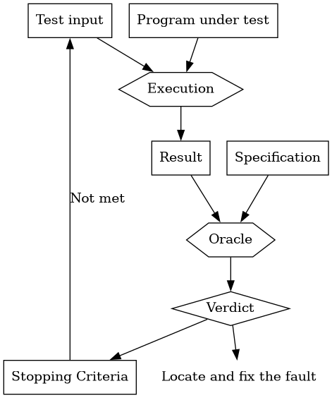
This diagram puts in evidence three main problems to be solved when designing our tests. First we need to identify a set of test inputs that will become the starting point for the tests cases. Then, for each test case we need to define a strong oracle able to tell when the result of the execution meets the requirements or not. Also we need to know how much should we test, that is, to set a stopping criterion. Ideally we would test until there are no more faults or when we explore all possible inputs, but this can not be done in practice. Locating and fixing an identified fault is also a very important problem, but it is out of the scope of testing and more related to debugging. However, tests failures should provide enough information for developers to find and correct the fault.
Solving these problems is far from easy. But, no matter the solution or strategy we pick, our ultimate goal should be to design tests capable of discovering faults.
3.4.1. Reachability, Infection, Propagation, Revealability
The main goal of testing is to reveal the presence of faults. However, there are four concrete conditions that a test case execution should meet to be able to discover a fault. These conditions are expressed in the Reachability, Infection, Propagation, Revealability (RIPR) model (57).
Listing 46 shows the findLast method. This method should return the index of the last occurrence of a given element in a given array. If the element is not present the method should return -1 and if the array is null it should throw an instance of NullPointerException. The method in question has a fault, the loop condition should be i >= 0 instead of i > 0. Due to this fault this findLast will never compare element to the value in the first position of the array.
findLast is supposed to return the index of the last occurrence of a given element in a given array. If the array is null the method should throw a NullPointerException exception. If the element is not present, then it should return -1. This method contains a fault as it never inspects the first element of the array.public static int findLast(int[] array, int element) {
for (int i = array.length - 1; i > 0 ; i--) { (1)
if(array[i] == element)
return i;
}
return -1;
}| 1 | Loop condition should be i >= 0. |
Listing 47, Listing 48, Listing 49 and Listing 50 show test cases exercising findLast. However, all these test cases fail to observe the bug for different reasons. We shall use these test cases to illustrate the concepts behind the RIPR model. We shall also discover how the model can explain why the fault is not discovered.
- Reachability
-
For a test case to discover a fault it must first execute/reach, the code location where the bug is present. The test case in Listing 47 tests the behavior of the method when the input array is
null. Therefore this test case never executes the loop condition and does not reach the fault.Listing 47. A test case that does not reach the fault.@Test public void testNull() { assertThrows(NullPointerException.class, () -> { findLast(null, 1); }); } - Infection
-
Reaching the location of the fault is not the only condition the execution should meet to discover the fault. The test case should also produce an incorrect program state, that is, it should infect the program state with incorrect values. Listing 48 fails to do that. In this test case the element in the first position of the array is never inspected. The last occurrence of the element given as input is found at the last position of the array. The test case has the same behavior in the presence of the fault as is the program was correct. On the other hand, Listing 49 do infect the state of the program. The first position is not checked in the faulty version which is not the case for the correct program. So, the infection comes for the fact
iis never0during the execution while it should have had this value at some point.Listing 48. A test case that reaches the location of the fault but does not infect the program state.@Test public void testLastElement() { int[] array = {0, 1, 2}; assertEquals(array.length - 1, findLast(array, 2)); } - Propagation
-
Listing 49 do infect the program but does not reveal the fault. A test case must reach the location of the fault, infect the program state but also propagate the program state infection to the rest of the execution. <Listing 49 produces an incorrect program state as the first position of the array is not inspected but returns the right result, so the error does not even reach the code of the test case. On the other hand, Listing 50 do propagate the infection to an observable code location. In this new test case
findLastproduces a wrong result. However, the test case is not yet able to detect the fault.Listing 49. A test case that reaches the fault, infects the program state but does not propagate the infection.@Test public void testNotFound() { assertEquals(-1, findLast(new int[]{0, 1, 2}, 4)); } - Revealability
-
It is impractical, if not impossible, to create an oracle that observes the entire program state. That is why, for a test case to discover a fault, it must not only reach the location, infect the program state and propagate the infection to the rest of the execution. The test must also observe the right portion of the state and use a strong condition to verify it. Listing 50 reaches the fault, infects the program state, produces a wrong result that propagates to the code of the test case, but the oracle is not adequate to reveal the fault. The assertion in the test case validates that no exception is thrown. The assertion does not verify the result of
findLast.Listing 50. A test case that fails to reveal the fault, due to a weak oracle. The method returns a wrong value-1when the correct value is0. The assertion inspects a different part of the program state.@Test void testExecutesNormally() { assertDoesNotThrow(() -> findLast( new int[]{0, 1, 2}, 0)); }Only the test case in Listing 51 meets all the conditions to reveal the fault in the method. The method produces an incorrect value,
-1, which is not the expected value0. When this new test case is executed all conditions are met. The fault is reached, the state is infected, the infection is propagated to the code of the test case, there is an oracle observing the right portion of the program state and the oracle is strong enough to make the test case fail with the wrong result.Listing 51. A test case able to reveal the fault.@Test public void testFirst() { assertEquals(0, findLast(new int[]{0, 1, 2}, 0)); }
Not all test cases should discover all faults. Test cases should remain simple as we discussed before. A single test case can not cover all possible execution scenarios and can not discover all potential faults. That is why a test suite should be conformed by many different test cases. These test cases should be carefully designed to select the right input able to reach faults, infect the program state and propagate the infection. Then, test cases need strong oracles to discover the fault. The design of a test suite should be guided by concrete criteria ensuring that these conditions if there is a fault. These criteria not only will ensure the creation of good test cases, they will also provide a concrete way to evaluate the quality of a test suite as a whole.
3.4.2. Coverage criteria for test qualification
Designing tests is hard. We need to choose good inputs to ensure potential faults are reached and that their effects do propagate to an observable point in the program execution. We also need to design strong oracles so the faults can be discovered and we need to know how many test cases our test suite should have to assure certain level of quality in the testing process.Formal Coverage criteria help testers solve these problems.
According to Ammann and Offutt [ammann2016introduction], a coverage criterion can be seen as a collection of rules that impose test requirements for a test suite. A test requirement is a specific element of a software artifact that a test case must satisfy or cover.
Perhaps the most widely used coverage criterion nowadays in industry is statement coverage. This coverage establishes each program statement as a test requirement, that is, it expects the test suite to execute all statements in the code of the program under test. So, following this criterion we create test cases until all statements are executed by the test suite.
In practice it is quite hard, sometimes not even desirable, that all test requirements of a coverage criterion are satisfied or covered by the test suite. For example, making test cases just to execute statements from simple getter methods might be a waste of resources.
A coverage criterion has a coverage level associated. The coverage level is the ratio of test requirements that are covered by the test suite. For statement coverage this is the percentage of statements in the program that are executed by the tests.
Coverage criteria help testers create more effective and efficient test suites, with fewer tests cases and better fault detection capabilities. Following coverage criteria we are able to better explore the input space. A coverage criterion ensures the traceability from each test case to the test requirements they cover. The purpose of a test case becomes, clear, as it is designed to cover a specific requirement or a specific set of requirements. Coverage criteria also set a well defined stopping condition for the test creation process and provide an effective way to evaluate the quality of the test suite.
The following sections introduce and explain some of the most relevant and known coverage criteria.
Input space partitioning
The input domain of a system under test is the set of all possible values that the input parameters can take. If there are more than one parameter, then the input domain is the cartesian product of the domains of all parameters. The input domain also includes values that could be incorrect for the program. These are also very important for testing purposes. A test input is then a tuple of values from the domain, one for each parameter.
For example, Listing 52 shows the signature of the findLast method introduced first in Listing 48. This method takes as input an array of integers and an integer. Therefore its input domain is a tuple of all possible integer arrays, including null and empty arrays and all possible integers. Test inputs for this method could be { array: null, element: 1 }, { array: {}, element: 2 }, { array: {1, 2, 3}, element: 4 }.
null array, an empty array and so on, and all possible integers.public static int findLast(int[] array, int element) { ... }Listing 53 shows the signature of a method that takes three integers and says if they form a valid date according to the Gregorian Calendar. The input domain is the set of all possible tuples of three integer elements, including negative integers and zero. Possible test inputs may include: { day: 1, month: 2, year: 200 }, { day: 19, month: 9, year: 1983 } or { day: 33, month: 12, year: 1990 }.
public static boolean isValidDate(int day, int month, int year) { ... }Listing 54 shows an extract of the BoundedStack class shown in Listing 33. In case we are testing methods push and pop, we should consider all possible values of elements and count. That is, when testing classes, instance fields, and even global static fields used by the method are also part of the input. Observe that in this case, elements will never be null since it is created in the constructor.
BoundedStack class presented in Listing 33. Observe that all values of the fields elements and count form part of the input domain for the push and pop methods.
class BoundedStack {
    private int[] elements;
    private int count;

    ...

    public void push(int item) {
        if(count == elements.length) {
            throw new IllegalOperationException();
        }
        count = count + 1;
        elements[count] = item;
    }

    public int pop(int item) {
        if(elements == 0) {
            throw new IllegalOperationException();
        }
        count = count - 1;
        return elements[count];
    }

    ...
}
The input space partitioning technique design tests based on a model of the input domain. From this model it is possible to derive several coverage criteria which result in a broad selection of potential test inputs. The technique uses only the interface of the program, the signature of the method or even the specification, but does not need to observe the internal structure of the artifact being tested. In this sense it is said to be a blackbox technique, as opposed to whitebox techniques, that heavily rely on the internal structure, for example, the code of the method.
To model the input, this technique creates partitions of the domain. A partition is a subdivision of the domain into subsets or blocks in such a way that the union of all blocks results in the entire input domain and all blocks are disjoint, that is, no element, or test input, can be included in more than one block for the same partition. Each partition is created by identifying characteristics which describe the structure of the input domain. Characteristics and blocks should be designed in such a way that all values in one block are equivalent according to the characteristic that defines the partition.
Identifying the right characteristics is hard and requires expertise. There are two main approaches: interface based modeling and functionality based modeling.
Interface based modeling considers each parameter separately and takes information only from their specific domain. It is a simple alternative that makes it easier to identify the characteristics. However, it does not use all the information available like the specification and fails to capture the interaction between parameters.
Using interface based modeling to describe the input of findLast from Listing 52 we may identify the characteristics shown in Table 4. Two characteristics are identified: `array` is null` and `array is empty. Each characteristic defines a partition with two blocks, one to contain the arrays for which the condition of the characteristic is true and another containing arrays for which the characteristic is false.
| Characteristics | Blocks | |
|---|---|---|
|
True |
False |
|
True |
False |
The same could be done in the parameter element, but it will not yield characteristics interesting enough for the tests. The values of element are irrelevant in isolation. It makes sense to look at them only in relation to the content of array.
Functionality based modeling uses semantic information and plays with the specification, the domain of each parameter and the interplay between the values of different parameters. Identifying good characteristics with this approach is harder but may yield better results.
For the same findLast method in Listing 52, with this approach we may identify the characteristics in Table 5. The table shows a characteristic that captures the number of times element appears in array which yields three blocks: one for arrays that do not contain element, one for arrays containing only one occurrence of element, and another for arrays in which element appears more than once. The other two characteristics consider the position of element in the array and each of them yields a partition with two block.
Characteristics |
Blocks |
||
Number of times |
0 |
1 |
> 1 |
|
True |
False |
|
|
True |
False |
|
Now we shall model the input of isValidDate from Listing 53. We first identify characteristics with the interface based approach. This may yield the following result:
Characteristics |
Blocks |
|
Value of |
<= 0 |
> 0 |
Value of |
<= 0 |
> 0 |
Value of |
<= 0 |
> 0 |
There is one characteristic for each parameter and they consider their values separately with respect to their domain. All possible values, valid or invalid are included and all blocks for the same characteristic are disjoint. Values close to the boundaries between valid and invalid inputs tend to be problematic and often source of bugs. So it is a good idea to include blocks reflecting these values. This way we can expand our initial characteristics as follows:
Characteristics |
Blocks |
||
Value of |
< 0 |
0 |
> 0 |
Value of |
< 0 |
0 |
> 0 |
Value of |
< 0 |
0 |
> 0 |
These blocks may be too broad for testing purposes. Sometimes it is useful to partition blocks into sub-partitions specially in the case of valid inputs.
In our example, the meaningful values of month and day depend on each other and the value of year. Actually, the number of valid days depend on the month, and even the year in the case of February, so we turn to a functionality based approach for new characteristics.
We first include the notion of leap year and subdivide years greater than 0 into leap and non-leap. Another almost equivalent solution for this could be to add a new characteristic reflecting this condition. We then include a block for valid month numbers and another for valid days which depend on the maximum valid number according to the month, represented as max(month, year).
Characteristics |
Blocks |
|||
Value of |
< 0 |
0 |
valid leap year |
valid non leap year |
Value of |
< 0 |
0 |
>= 1 and <= 12] |
> 12 |
Value of |
< 0 |
0 |
>= 1 and <= max( |
> max( |
We can go further and sub-partition valid month numbers into groups matching the maximum number of days on each. The result would be as follows:
Characteristics |
Blocks |
||||||
b1 |
b2 |
b3 |
b4 |
b5 |
b6 |
||
|---|---|---|---|---|---|---|---|
q1 |
Value of |
< 0 |
0 |
valid leap year |
valid common year |
||
q2 |
Value of |
< 0 |
0 |
{ 1, 3, 5, 7, 8, 10, 12} |
{ 4, 6, 9, 11 } |
2 |
> 12 |
q3 |
Value of |
< 0 |
0 |
>= 1 and <= max( |
> max( |
||
Now we have a block for months with 31 days, another for months with 30 days and one for February which is a very special case.
| Notice that this is not the only input model that we can design, and it might not even be the optimal. For example, it could be argued that, for this particular method, the blocks where each parameter is zero is equivalent to the blocks where each parameter is negative. There is no silver bullet when it comes to modeling the input. That is why experience and knowledge about the application domain are so important here. |
If the input contains a parameter with a enumerative domain of a few values, it could make sense to create a partition with one block per value. In our example we could have one block for each month, but there is no substantial different among months with the same amount of days for this particular method we are testing.
It should be taken into account that, when testing classes, different methods of the same class could share the same characteristics to define partitions. For example, both the push and pop methods in the stack implementation shown in Listing 33 could partition the input considering when the stack is empty or not. Therefore it is a good idea, when testing a class, to first find the characteristics for all methods and reuse them.
Once the features and blocks have been identified, the concrete test inputs are built by picking values matching a selection of blocks from different partitions. For example: {day: 1, month: 2, year:2000} is an input matching the third block for each of the partitions identified in Table 6, that is, blocks q1b3, q2b3`and `q3b3.
Test inputs can be immediately translated to concrete test cases. For example, if we select blocks q1b4, q2b5 and q3b4 we can pick { day: 29, month: 2, year: 2019}. The test case could be written as follows:
@Test
public void test29DaysFebruaryCommonYear () {
    assertFalse(isValidDate(29, 2, 2019), "February in common years should not have more than 28 days.");
}
Notice how designing test cases from block selections makes the test case clear and helps trace it back to the requirements.
The challenge now is to create effective block combinations. For that we can use the following coverage criteria:
- Each choice coverage (ECC)
-
This criterion sets each block from each partition as a test requirement. That is, we must select a set of inputs in such a way that all blocks are represented at least once.
The following set of inputs achieve ECC coverage. All blocks from Table 6 are covered by at least one input:
Input |
Blocks |
|
|
|
|
|
|
|
|
|
|
|
|
Sometimes it is not feasible to select certain blocks at the same time. For example, we should not pick q3b3: day larger than the maximum according to month and year, if month does not have a valid value, for example if we pick q2b1. Such combinations can be dropped when creating test inputs. However, if an input model contains too many of these restrictions it might be a good idea to redesign the partitions.
While this coverage criterion is easy to achieve, it may not yield good results, as it may miss interesting combinations between blocks.
- All combinations coverage (ACoC)
-
As a counterpart to ECC, to meet this criterion we must combine all blocks from all characteristics. This could lead to a very high number of combinations making it impractical. So fewer combinations are desirable. For partitions in Table 6 this criterion yields 82 test requirements or combinations after dropping unfeasible block selections.
- Pair-wise coverage (PWC)
-
Instead of all combinations, a value from each block, for each partition must be combined with a value from every block for each other partition. That is, all pair of blocks from different partitions are selected as test requirements. For partitions in Table 6 this criterion produces 62 test requirements, which can be covered by only 25 inputs. The number of inputs could still be high for some partitions.
An extension of PWC is to combine T characteristics or partitions at the same time (aka. T-wise test case generation), but it has been shown that this does not produce any improvement in practice.
Combining more than one invalid value is not useful in general. Most of the times, the program recognizes only of them and the effects of the others are masked. The following two criteria provide a good alternative to avoid that and produce a smaller number of inputs.
- Base choice coverage (BCC)
-
A base choice block is chosen for each partition or characteristic. A base test is formed with the base choice for each partition. Subsequent test inputs are formed by changing only one base choice from this base test and replacing it with another non-base block for the same partition and keeping the others. Base choices should always be the simplest, smallest, most common choices.
- Multiple base choice coverage (MBCC)
-
It is an extension of the previous criterion. This criterion may select more than one base choice for each partition. An initial test set is built using an ECC coverage on the base choices, then subsequent inputs are formed in the same way as in BCC: by replacing one base choice for another non-base block in the same partition and keeping the others.
For partitions in Table 6, we can pick q1b3 and q1b4 as base choices for the first characteristic, q2b3, q2b4, q2b5 for the second and q3b3 for the third one. With this setup we could pick the following inputs covering base choices: { day: 1, month: 3, year: 2019 }, { day: 30, month: 9, year: 2018 }, { day: 29, month: 2, year: 2020 }. Then, more inputs could be added by exchanging one basic block by another non-basic choice. For example, if we take { day: 29, month: 2, year: 2020 }, it matches blocks q1b4, q2b5 and q3b3. Changing q3b3 by q3b4 implies to change the value of day to a value larger than the maximum according to the month. With this we could change 29 by 30 and obtain a new input { day: 30, month: 2, year: 2020 }. The process continues until no new inputs can be added.
Input space partitioning helps defining an initial set of tests inputs. However, the criteria explained in this section do not ensure any of the conditions to discover a fault as stated by the RIPR model.
Structural coverage
As their name implies, structural coverage criteria rely on the internal structure of the artifact under test, that is, the code of the method, class or complete program we are testing. This section present some of the more commonly used criteria in this category.
- Statement coverage
-
The simplest structural criterion is statement coverage. This criterion establishes each statement in a program as a test requirement, that is, the test suite should be designed in such a way that all statements in the program are executed by at least one test case. In this way it ensures the reachability of the RIPR model. If all statements are covered, then all potential faults will be reached.
It is a simple criterion, easy to interpret and also very easy and fast to compute. Nowadays, most practitioners use the statement coverage level, that is, the ratio of statements executed by the test suite as a proxy for the quality of their tests. The practice is so common that the statement coverage level is known as code coverage or simply coverage. There are many available tools to compute code coverage and they are supported by most mainstream IDEs and CI/CD servers.
Listing 55 highlights the statements executed/covered/reached by the test case shown in Listing 48 on the code of the method included in Listing 46. With coverage information it is easy to see that, in the absence of more test cases, we miss a test where the element could not be found in the array, as the last statement is not executed.
Listing 55. Statements covered by the test case in Listing 48 on the code of the method from Listing 46.1 2 3 4 5 6 7 8
public static int findLast(int[] array, int element) { for (int i = array.length - 1; i > 0 ; i--) { if(array[i] == element) return i; } return -1; }
The last statement can be covered by a test case such as the one shown in Listing 49. Listing 56 highlights the statements covered by this test case on the code from Listing 46.
Listing 56.1 2 3 4 5 6 7 8
public static int findLast(int[] array, int element) { for (int i = array.length - 1; i > 0 ; i--) { if(array[i] == element) return i; } return -1; }
Notice that both test cases together cover all the instructions of the method. However they are not able to discover the fault. This criterion ensures reachability but does not ensure any of the other conditions for the fault to be found. It is extremely useful to rapidly known which pieces of code haven’t been tested but is not a good quality metric for a test suite.
Other structural criteria can be defined over the control flow graph of a method or a sequence of instructions. Recalling the procedure explained in [cyclomatic], the control flow graph of a method is built as follows:
-
Initially, the graph has two special nodes: the start node and the end node.
-
A sequence of instructions with no branches is called a basic block. Each basic block becomes a node of the graph.
-
Each branch in the code becomes an edge. The direction of edge coincides with the direction of the branch.
-
There is an edge from the start node to the node with the first instruction.
-
There is an edge from all nodes that could terminate the execution of the code, to the end node.
Figure 14 shows the control flow of the findLast method presented in Listing 46.
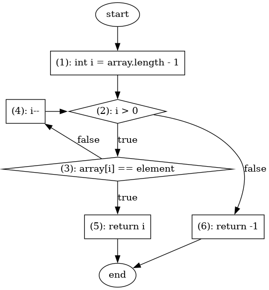
findLast method, presented in Listing 46.The execution of a test case produces an execution path or execution test over the control flow graph. This path goes from the start node to the end node and includes all nodes containing instructions executed by the test case and all edges connecting those nodes.
For example, the test case in Listing 48 produces the following path start ⇒ (1) ⇒ (2) ⇒ (3) ⇒ (5) ⇒ end. With this path, the test case covers the nodes/blocks (1), (2), (3) and (5). Nodes start and end are covered by all execution paths. The same path covers edges start ⇒ (1), (1) ⇒ (2), (2) ⇒ (3), (3) ⇒ (5), (5) ⇒ end. The test does not cover nodes (4) and (6) and edges (3) ⇒ (4), (4) ⇒ (2), (2) ⇒ (6) and (6) ⇒ end. Figure 15 shows in blue the elements covered by this test case in the graph.
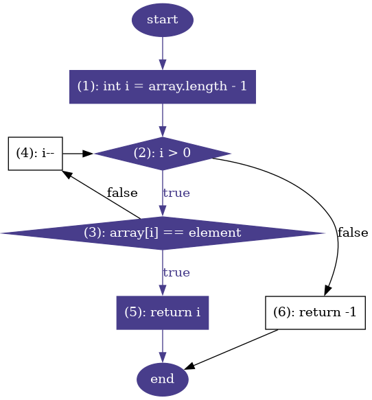
The following coverage criteria are precisely defined over the nodes, edges and paths of a control flow graph.
- Block coverage
-
With block coverage we consider each basic block or control flow graph node as a test requirement. This is very related to statement coverage, as basic blocks guarantee that if one instruction from the block is executed, all the other instructions in the same block will be executed as well. In fact, some tools actually compute block coverage to report statement coverage. In the example discussed before, the test from Listing 49 was able to cover all blocks but nodes
(4)and(6). - Branch coverage
-
This criterion sets branches in the program, that is, edges in the control flow graph as test requirements. Instead of the nodes, here we consider the edges in the execution paths. It helps determine whether all outcomes from decision branches have been explored by the test cases. In the example discussed before, the test from Listing 49 was able to cover all edges but
(3) ⇒ (4),(4) ⇒ (2),(2) ⇒ (6)and(6) ⇒ end. - Path coverage
-
This criterion sets all possible execution paths as test requirements. That is, we aim to design a test suite that traces all execution paths in the control flow graph. Executing all possible paths leads to exhaustive testing, and this is, however ideal, not possible in practice. For example, if the control flow graph contains a loop as in Figure 14 the number of possible execution paths is infinite. Therefore, we need to select which paths to cover in practice. The two following criteria are examples of how to select which paths to execute.
- Path basis testing
-
A directed graph is said to be strongly connected if for every pair of nodes we can find a path that starts in the first node and ends in the second node. A control flow graph can be made strongly connected if we add a bogus edge from the end node to the star node. A circuit in a graph is which ends at the same node it begins.
If we add the bogus edge, the execution of the test case in Listing 48 produces the circuit
start ⇒ (1) ⇒ (2) ⇒ (3) ⇒ (5) ⇒ end ⇒ start.A set of circuits from a graph is said to be linearly independent if all of the circuits differ in at least one edge. This set of circuits is said to be a basis for all circuits in the graph if all edges are included in at least one circuit from the set. All circuits in the graph can be formed by combining circuits in the base.
If a directed graph is strongly connected, then, the cyclomatic complexity, as discussed in Section 2.1.3.2, is equal to the maximum number of linearly independent circuits, that is, the number of circuits in the base. The basis is not unique. In general we can find more than one basis for the same graph.
For the graph in Figure 14 the number of circuits in the basis is 3 which is the number of conditionals: 2 plus 1. The following could be a basis of circuits:
-
start ⇒ (1) ⇒ (2) ⇒ (3) ⇒ (5) ⇒ end ⇒ start -
start ⇒ (1) ⇒ (2) ⇒ (6) ⇒ end ⇒ start -
(2) ⇒ (3) ⇒ (4) ⇒ (2)
If we set all linearly independent circuits as test requirements, then we create a test for each circuit in the base and we ensure that we are testing, at least once, each outcome from a decision or conditional node. For example, the test case in Listing 48 covers the first circuit in the basis, in which the element appears in the last position. Testing with an empty array would cover the second circuit in the basis. Any test case that loops over the array covers the third and last circuit in the basis, such as the test case in Listing 49. See that with these three test cases we are able to cover the entire basis but we still do not reveal the fault.
-
The cyclomatic complexity sets a lower bound for the number of different tests executing all branches. In this example the cyclomatic complexity is 3 which is also the number of test cases that cover the basis.
- Prime path coverage
-
A simple path in a graph is a path where no node appears more than once, except perhaps the first node, that could be also the last one. A prime path in a graph is a simple path that is no proper sub-path of any other simple path. This means that a prime path is a simple maximal path.
In Figure 14
(2) ⇒ (3) ⇒ (4) ⇒ (2)is a prime path that starts and ends in(2). Computing all prime paths from a graph is simple. We start with all edges, which are simple paths of length one. From there we form more simple paths by adding edges until we reach the initial node, there are no more edges to add or the next node already appears somewhere in the path. Finally, we keep the paths that are no proper sub-paths of any other. For the graph of the example the prime paths are:-
start ⇒ (1) ⇒ (2) ⇒ (3) ⇒ (5) ⇒ end -
start ⇒ (1) ⇒ (2) ⇒ (6) ⇒ end -
start ⇒ (1) ⇒ (2) ⇒ (3) ⇒ (4) -
(4) ⇒ (2) ⇒ (3) ⇒ (5) ⇒ end -
(3) ⇒ (4) ⇒ (2) ⇒ (6) ⇒ end -
(2) ⇒ (3) ⇒ (4) ⇒ (2) -
(4) ⇒ (2) ⇒ (3) ⇒ (4) -
(3) ⇒ (4) ⇒ (2) ⇒ (3)
Prime path coverage sets each prime path as a test requirement. That is, at least one test case should cover each prime path. For example, Listing 48 covers the first prime path of the list. The test case in Listing 49 produces the following path:
start ⇒ (1) ⇒ (2) ⇒ (3) ⇒ (4) ⇒ (2) ⇒ (3) ⇒ (4) ⇒ (2) ⇒ (6) ⇒ end. This test traces the entire array and does not find the element. It is able to cover prime paths 3, 5, 6, 7 and 8 from the list above. This criterion is useful when testing loops in a program. It ensures the creation of tests cases that skip the loops and test cases that execute several iterations of each loop. In our example, prime path 2 corresponds to a scenario where theforloop is never entered, i.e.arrayis empty. The execution of prime paths 6, 7, 8 produces tests performing more than one iteration. -
Many software artifacts can be represented as graphs. As an example, Finite State Machines are a special type of graph that have been widely used to represent the behavior of software elements. Actually, most embedded software is modeled as a state machine. Finite state machines can also be used to describe specifications for software and even how a user interface should behave.
In a finite state machine, a node represent a state of the artifact and edges represent changes in those states. As an example, recall Figure 5 where a state machine was used to model the behavior of a microwave oven.
The structural criteria defined over the control flow graph of a method can be extended to any type of graph. Branch coverage can be generalized as edge coverage and block coverage is just a special case of node coverage. In the particular case of finite state machines, designing test cases to achieve edge coverage ensures that all state transitions are explored and targeting node coverage ensures that all possible states of the artifact have been observed in at least one test case.
But, as explained before, the structural criteria discussed in this section only ensure that most parts of the software under test are executed. Therefore they guarantee that, if there is a fault, it will be executed by at least one test case. However, these criteria do not ensure that the input will infect the program state, or that the effects will be propagated to an observable point or that there will be an oracle strong enough observing the right portion of the state.
Logic coverage
A predicate is a boolean expression. They are used in all kinds of software. Predicates define branches in source code and also define the state of finite state machines like the microwave oven in Figure 5.
The coverage criteria presented in this section are designed specifically for predicates. They are also designed in such a way that, if there is a fault, test cases created with the help of these criteria guarantee that the state of the program will be, at least, infected by the fault. This means that, if there is a fault in the code of the predicate, there will be at least one test case where the predicate will produce the wrong result.
A predicate is defined as follows:
-
A clause is a predicate. Clauses are the shortest predicates. They are the simplest boolean expressions that do not contain logical operators. They can be:
-
a variable reference i.e. \$a\$
-
a comparison or any other relational expression i.e \$a < 3\$, \$a = b\$
-
a function call i.e. \$f(a, b+3)\$
-
-
If \$p\$ and \$q\$ are predicates, then the following are also predicates:
-
\$\neg p\$ (negation)
-
\$p \wedge q\$ (conjunction)
-
\$p \vee q\$ (disjunction)
-
\$p \implies q\$ (implication)
-
\$p \iff q\$ (equivalence)
-
\$p \oplus q\$ (exclusive disjunction)
-
\$ a < 3 \vee c \implies fn(b)\$ is a predicate with three clauses: \$a < 3\$, \$c\$ and \$fn(b)\$.
Listing 57 shows the isLeapYear method which implements a predicate to determine if a given integer represents a leap year or not. The predicate has three clauses, \$c_400\$: year % 400 == 0, \$c_4\$ year % 4 == 0 and we conveniently represent year % 100 == 0 as \$c_100\$ \$c_100\$: year % 100 == 0 negated. In this example the clauses are not independent from each other. Also, given the short-circuit behavior of logical operators in most programming languages, the order in which the clauses are evaluated play a role in the evaluation of the predicate.
public static boolean isLeapYear(int year) {
    return year % 400 == 0 || ( year % 4 == 0 && year % 100 != 0 );
}
The simplest logic coverage criteria sets test requirements according to the value that takes the predicate as a whole and the value of each clause.
- Predicate Coverage (PC)
-
This coverage criterion sets two test requirements: one on which the predicate evaluates to
trueand another where the predicate evaluates tofalse.To fulfill this criterion we require only two inputs one making the predicate
trueand another making the predicatefalse. It is a simple criterion but the clauses are not considered individually. Taking the predicate, \$((a > b) \wedge C) \vee p(x)\$ we can cover both requirements with \$(a = 5, b = 4, C = true, p(x) = true)\$ and \$(a = 5, b = 4, C = false, p(x) = true)\$, however, in both interpretations, the first and last clauses of the predicate have always the same value. - Clause Coverage (CC)
-
This criterion sets two test requirements for each clause in a predicate. For one requirement, the selected clause should be
trueand for the other the same clause should be falsefalse.For the predicate \$((a > b) \wedge C) \vee p(x)\$ we have six requirements, two for each clause. The criterion can be covered using the following two sets of values: \$(a = 5, b = 4, C = true, p(x) = true)\$ and \$(a = 5, b = 6, C = false, p(x) = false)\$. The first set of values covers all requirements where clauses are
trueand the second covers the scenarios where the clauses evaluate tofalse. So, with only two inputs it is possible to cover all six requirements.This criterion does enforce combinations between the clauses. Also, it is possible to fulfill clause coverage and not predicate coverage at the same time. Take as example the predicate \$a \vee b\$. Using \$a = true, b = false)\$ and \$(a = false, b = true)\$ we can cover all clauses but the predicate always evaluates to
true. - Combinatorial Coverage (CoC)
-
This criterion sets a test requirement for each combination or truth value of all clauses.
For example, for the predicate \$[((a > b) \wedge C) \vee p(x)\$] we create the following test requirements:
\$a > b\$ \$C\$ \$p(x)\$ \$((a > b) \wedge C) \vee p(x)\$ truetruetruetruetruetruefalsetruetruefalsetruetruetruefalsefalsefalsefalsetruetruetruefalsetruefalsefalsefalsefalsetruetruefalsefalsefalsefalseThis criterion accounts for any truth value combination of all clauses and ensures all possible values for the predicate. However, it is not feasible in practice for large predicates. The number of requirements is exponential with respect to the number of clauses in the predicate, that is we have \$2^N\$ requirements for \$N\$ clauses.
So, we need a set of criteria able to evaluate the effects of each clause over the result of the predicate while keeping the number of test requirements reasonable low.
- Active Clause Coverage
-
This criterion verifies each clause under conditions where they affect the value of the entire predicate. When we select a clause, we call it a major clause and rest are called minor clauses. So when defining the requirements for this criterion each clause become major at some point.
A major clause determines the predicate if the minor clauses have values such that changing the truth value of the major clause also changes the value of the predicate.
For the predicate \$((a > b) \wedge C) \vee p(x)\$ if we select \$a > b\$ as the major clause, \$C\$ and \$p(x)\$ are the minor clauses. If we assign values \$(C = true, p(x) = false)\$ to the minor clauses, \$a > b\$ determines the predicate because, when the major clause is
truethe entire predicate istrueand when the major clause isfalsethe predicate evaluates tofalse.This criterion selects each clause in the predicate as a major clause. Then, for each major clause \$c\$, we select values for the minor clauses in a way that \$c\$ determines the predicate. Then the criterion sets one test requirement for \$c = true\$ and another for \$c = false\$.
For example, for the predicate \$p = a \vee b\$ is easy to see that each clause determines the predicate when the other is
false. So, selecting \$a\$ as the major clause we obtain requirements \$(a = true, b = false)\$ and \$(a = false, b = false)\$. We proceed in a similar way with clause \$b\$ and obtain \$(a = false, b = true)\$ and \$(a = false, b = false)\$. One of the requirements is common for both clauses, so in the end we have three test requirements \$(a = true, b = false)\$, \$(a = false, b = true)\$ and \$(a = false, b = false)\$.A major challenge for the active clause criterion is the handling of the minor clauses. We need first to obtain the possible values for the minor clauses to make the major clause determine the predicate.
Given a predicate \$p\$ and a major clause \$c \in p\$, the predicate \$p_c = p_{c=true} \oplus p_{c=false}\$ represents the condition for \$c\$ to determine \$p\$. That is, the values of the minor clauses that make \$p_c\$ be
truealso make \$c\$ determine \$p\$.The following examples illustrate how to use this result to find the values for the minor clauses.
The following examples make heavy use of Boolean Algebra. It would be better to refresh the main rules before going any further. Take the predicate \$p = a \vee b\$, selecting \$a\$ as the major clause we need to find a condition for \$b\$ so \$a\$ dominates the predicate. We proceed as follows:
\[\begin{eqnarray*} p_a & = & p_{a=true} \oplus p_{a=false} \\ & = & (true \vee b) \oplus (false \vee b) \\ & = & true \oplus b \\ & = & \neg b \end{eqnarray*}\]Which means that \$a\$ determines the predicate, only when \$b\$ is
false.Let’s take now the predicate \$p = a \wedge (b \vee c)\$ and again \$a\$ as the major clause. We obtain:
\[\begin{eqnarray*} p_a & = & p_{a=true} \oplus p_{a=false} \\ & = & (true \wedge (b \vee c)) \oplus (false \wedge (b \vee c)) \\ & = & (b \vee c) \oplus false \\ & = & (b \vee c) \end{eqnarray*}\]This means that any values for \$b\$ or \$c\$ making \$b \vee c\$
truewill also make \$a\$ determine \$p\$. In this case we could use \$(b = true, c = true)\$, \$(b = false, c = true)\$ or \$(b = true, c = false)\$.On another example, if we take \$p = a \iff b\$, we obtain:
\[\begin{eqnarray*} p_a & = & p_{a=true} \oplus p_{a=false} \\ & = & (true \iff b) \oplus (false \iff b) \\ & = & b \oplus \neg b \\ & = & true \end{eqnarray*}\]We observe that \$p_a\$ is always
true. Therefore, \$a\$ determines \$p\$ no matter the value of \$b\$. On the other hand, it could be that \$p_a\$ would result infalse. In that case it would be impossible for the clause \$a\$ to determine \$p\$.As seen in the examples above, we can obtain four possible outcome when finding the condition for a major clause to determine the predicate: (1) the clause can not determine the predicate, (2) there is only one possible assignment (also known as interpretation) for the values of the minor clauses, (3) there is more than one possible interpretation and (4) the clause always determines the predicate.
ACC sets two test requirements for each major clause: one in which the clause is
trueand another in which the clause isfalse. If there is more than one possible interpretation for the minor clauses we may decide to use different values on each requirement or force the same values of the minor clauses. If we force the use of the same values for the minor clauses, then we are using what is known as Restricted Active Clause Coverage (RACC). This is a stronger criterion but it can not be always satisfied when clauses are not independent.
In fact, it could be possible that a test requirement becomes infeasible due to dependencies between the clauses for any of the previous coverage criteria. Given the case, we simply discard those inputs.
The literature often describes Modified Condition/Decision Coverage (MC/DC). This coverage criterion is defined as follows (58):
Every point of entry and exit in the program has been invoked at least once, every condition in a decision in the program has taken all possible outcomes at least once, every decision in the program has taken all possible outcomes at least once, and each condition in a decision has been shown to independently affect that decision’s outcome. A condition is shown to independently affect a decision’s outcome by varying just that condition while holding fixed all other possible conditions.
In this definition, a decision is a predicate and a condition is a clause. Therefore, achieving RACC for all predicates in a program ensures MC/DC.
Now, we use ACC to derive test requirements for the method in Listing 57. We rewrite the predicate encoded in the method as \$p = c_400 \vee (c_4 \wedge \neg c_100)\$, where \$c_x\$ is equivalent to year % x == 0.
Selecting \$c_400\$ as the major clause we obtain \$p_{c_400} = \neg c_4 \vee c_100\$. The following table shows the values, or interpretations of the clauses that make \$p_{c_400}\$ true.
| \$c_4\$ | \$c_100\$ | \$p_{c_400}\$ |
|---|---|---|
|
|
|
|
|
|
|
|
|
But, these clauses are not independent. In fact the first row of the table is not feasible. The same number can not be divisible by 100 (\$c_100 = true\$) and not by 4 (\$c_4 = false\$). Therefore we throw it away and keep only the two last rows, which leads us to the following truth values for \$p\$:
| \$c_400\$ | \$c_4\$ | \$c_100\$ | \$p\$ |
|---|---|---|---|
|
|
|
|
|
|
|
|
|
|
|
|
|
|
|
|
Again, the clauses are not independent in this example. The fourth row also lead to and impossible situations so we keep only the rest.
| \$c_400\$ | \$c_4\$ | \$c_100\$ | \$p\$ |
|---|---|---|---|
|
|
|
|
|
|
|
|
|
|
|
|
For this clause we can pick the the first and second rows to satisfy RACC.
Now we select \$c_4\$ as the major clause and obtain \$p_{c_4} = \neg c_100 \wedge \neg c_400\$ which is true only for the following interpretation:
| \$c_100\$ | \$c_400\$ | \$p_{c_4}\$ |
|---|---|---|
|
|
|
Therefore, we obtain the following two additional test cases:
| \$c_400\$ | \$c_4\$ | \$c_100\$ | \$p\$ |
|---|---|---|---|
|
|
|
|
|
|
|
|
Finally we pick \$c_100\$ as the major clause obtaining \$p_{c_100} = \neg C_400 \wedge c_4\$. The only possible interpretation to make \$c_100\$ dominate the predicate is:
| \$c_400\$ | \$c_4\$ | \$p_{c_100}\$ |
|---|---|---|
|
|
|
Which leads to the following test cases:
| \$c_400\$ | \$c_4\$ | \$c_100\$ | \$p\$ |
|---|---|---|---|
|
|
|
|
|
|
|
|
Some of the test cases for different clauses are the same, so we combine them and obtain as final requirements the following inputs:
| \$c_400\$ | \$c_4\$ | \$c_100\$ | \$p\$ |
|---|---|---|---|
|
|
|
|
|
|
|
|
|
|
|
|
|
|
|
|
In the end we have created four different test cases. Ensuring ACC, also ensures PC and CC and produces fewer tests than CoC while observing the effect of each clause.
The inputs created above have to interpreted with respect to year which is the actual parameter of the method and defines the value of all clauses and their relationship. To satisfy the first requirement in the table above we need a value that is divisible by 4, 100 and 400 at the same time, which actually means that we need a value divisible by 400 as it implies the other two conditions. For the second requirement we need a value divisible by 100 but not by 400. The third row requires a value not divisible by 4 and the last needs one divisible by 4 but not by 100. The following table summarizes the result:
| \$c_400\$ | \$c_4\$ | \$c_100\$ | \$p\$ | year |
|---|---|---|---|---|
|
|
|
|
2000 |
|
|
|
|
1900 |
|
|
|
|
2017 |
|
|
|
|
2020 |
Here we picked values that resemble recent years to be closer to the intention of the method. We could have picked, 400, 100, 3 and 4 as well but these values are not so intention revealing as the others.
Mutation testing
We can use the coverage criteria studied so far to select meaningful sets of test inputs, to create test cases able to reach most potential faults and even to guarantee the program state infection for predicates. However, they do not ensure the creation of test cases able to reveal faults. In particular they do not consider the propagation and revealability conditions of the RIPR model. As an extreme example, we could remove all the assertions in a test suite. The test suite will be able to cover the same number of statements as before while it will loose its ability to evaluate the result of the tests. See for instance, that removing the assertion invocation in Listing 51 leaving the method invocation, will produce the same coverage for findLast, but it will not uncover the fault anymore. Statement coverage, is useful to discover the code that is not tested but it is not good when it comes to evaluate the capability of the test suite to reveal bugs, which is, in the end, the main purpose of testing.
Mutation testing or mutation analysis is a coverage criterion that directly assesses the capability of a test suite to discover bugs. It was first proposed in by DeMillo et.al. in the late 70’s of the last century (59).
The idea behind this criterion is simple: if a test suite should reveal bugs, then we can assess how effective it is by using artificial faults. That is, we insert artificial faults in the program and then we execute the test suite for each fault. The test suite should fail under these conditions, otherwise it needs to be improved.
By inserting the artificial fault we mutate the original program to create a faulty version. This version is called a mutant. If there is at least one test case in the test suite that fails when it is executed with the mutant, then the mutant is considered as detected and it is said to be killed. Otherwise it is a live mutant. As a coverage criterion, mutation testing targets all live mutants as test requirements. This means that we design test cases to fail with those mutants that are not detected by the current set of test cases.
The mutation score is the ratio of killed mutants to the total number of mutants used. It is the the coverage level for this criterion and it is often used to quantitatively evaluate the bug revealing capabilities of a test suite. We aim to design test suite with high mutation score.
In general, mutation testing works under following two assumptions:
-
Programmers create programs that are close to being correct (The competent programmer hypothesis) and
-
A test suite that detects all simple faults can detect most complex faults. That is, complex errors are coupled to simple errors. (The coupling effect)
So, to create a mutant, mutation testing inserts only small and well localized syntactic changes. These changes follow predefined fault or transformation models called mutation operators. A mutation operator could, for example, change + by - in an arithmetic expression. Other operators may change a comparison operator, for example > by >=, change a constant in the code, for example, change any constant by 0, remove a method invocation and so on.
[mutation-testing-algorithm] shows in pseudo-code how mutation testing works. The procedure takes as input a program under test, the test suite designed to verify the program and a set of mutation testing operators. All mutation operators are used to create a set of mutants. Each mutant is then challenged against the test suite. If the test suite does not fail when executing a mutant, the faulty program version is kept as a live mutant. In the end, the procedure reports the list of live mutants and the mutation score.
input: program, test_suite, mutation_operators
ouput: live_mutants, mutation_score
procedure:
    live_mutants = {}
    for mutant in generate_mutants(program, mutation_operators): (1)
        fails = execute(test_suite, mutant) (2)
        if not fails:
            live_mutants.append(mutant)
    mutation_score = 1 - size(live_mutants)/size(mutants)
return live_mutants, mutation_score (3)| 1 | Create mutants based on the mutation operators. |
| 2 | Execute the entire test suite with the mutant. fails is false if no test case failed in the execution. |
| 3 | The procedure returns the set of live mutants and the mutation score. |
To illustrate the functioning of mutation testing we go back to the code of Listing 33. We will consider the BoundedStack class as the program under test. Listing 59 shows the test suite we shall evaluate with the help of mutation testing. This test suite contains only two test cases: one verifying the push method and another verifying the pop method.
public class BoundedStackTest {
    @Test
    public void testPush() {
        BoundedStack stack = new BoundedStack(1);
        stack.push(1);
        assertEquals(1, stack.size());
    }

    @Test
    public void testPop() {
        BoundedStack stack = new BoundedStack(1);
        stack.push(1);
        stack.pop();
        assertEquals(0, stack.size());
    }
}
We use the following four mutation operators:
-
Negate the boolean expression of conditional statements.
-
Replace
+by-in arithmetic expressions. -
Replace
-by+in arithmetic expressions. -
If a method returns an integer, we change the return value by
0.
Listing 60 shows the same BoundedStack class as in Listing 33 and highlights are the locations where the artificial faults are inserted to create the mutants.
BoundedStack shown in Listing 33.public class BoundedStack {
private int[] elements;
private int count;
public BoundedStack(int capacity) {
elements = new int[capacity];
count = 0;
}
public void push(int item) {
if(count == elements.length) { (1)
throw new IllegalStateException();
}
elements[count] = item;
count = count + 1; (2)
}
public int pop() {
if(count == 0) { (3)
throw new NoSuchElementException();
}
count = count - 1; (4)
return elements[count]; (5)
}
public int size() {
return count; (6)
}
public int capacity() {
return elements.length; (7)
}
}| 1 | Negate the conditional: count != elements.length. |
| 2 | Replace + by -: count = count - 1. |
| 3 | Negate the conditional: count != 0. |
| 4 | Replace + by -: count = count + 1. |
| 5 | Replace the result by 0: return 0. |
| 6 | Replace the result by 0: return 0. |
| 7 | Replace the result by 0: return 0. |
With the four mutation operators we obtain seven mutants in total. Two mutants, (<1> and <3>) are produced by negating conditionals inside push and pop. A mutant (<2>) is produced by changing the arithmetic operator in the increment inside push and another by changing the decrement inside pop (<4>). The other three are created by changing the result of pop, size and capacity. No fault was inserted in the constructor of the class.
Now, each fault is inserted in isolation from the rest and that each mutant is challenged by the execution of the test suite. The outcome for each mutant is as follows:
-
Mutant 1 is killed. It makes
popthrow an unexpected exception which also makes both test casestestPushandtestPopfail. -
Mutant 2 is killed. After the fault is executed,
countresults in-1then the assertion intestPushfails as it expects the result ofsizeto be 1 and not-1; -
Mutant 3 is killed in the same way as mutant <1>:
popthrows an unexpected exception andtestPopfails. -
Mutant 4 is killed. At the end of the invocation of
popintestPop,countis equal to2which is not the expected value per the assertion and the test case fails. -
Mutant 5 lives. It is not detected by any of the two test cases. In the code of the mutant
popreturns0. However, thetestPopdoes not verify the result of the method. Therefore the test case does not fail and the mutant lives. -
Mutant 6 is killed. The result of
sizechanged to return0. This does not maketestPopfail but it does maketestPushfail as the expected value is1. -
Mutant 7 lives. The method is not invoked by any test case, therefore the mutated code is never reached and the mutant lives.
Out fo the seven mutants, two survived the analysis. Then, this small test suite has a score of \$\frac{5}{7}\$. Inspecting both live mutants we can find hints on how to improve our test suite.
The fault introduced to create mutant 7 is not executed by the test suite. In this sense we say that the mutant is not reached by the test suite. capacity is a simple getter, it might be a waste of time to create a test case only to verify it but it exposes part of the internal state of a BoundedStack instance. The fact that it is not executed means that we are not verifying this part of the state. So, instead of creating a test case designed to check the functionalities of capacity it might be better to check that the other methods do not affect the part of the state that capacity exposes. In the case of our example we might verify that the capacity of the stack never changes. See that unreached mutants produce the same information as code coverage.
On the other hand, mutant 5, is reached by the test suite. The artificial fault actually infects the program state as the result of pop is changed in the execution from 1 to 0. However the oracle in testPop does not check the result of pop and it becomes evident that we should either add a new assertion for this or even create a new test case designed to check the result of the method.
Mutation testing evaluates the test suite as a whole. So, it is not required to improve testPop to detect mutant <6> as it is detected by testPush. In the same way no test case can cover all scenarios, all test cases shall not kill all mutants.
Although it has gained some attention in the last few years and in spite of being several decades old, mutation testing has still a scarce adoption in industry when compared with code coverage. The main reason for that lay in the limitations of the criterion:
-
The mutation testing process is complex. There is a true lack of tooling support with easy integration in the development process beyond academic circles. However, this has changed with the emergence of industrial level tools like PIT, for Java programs (60).
-
Mutation testing is very expensive in terms of execution time. This is one of the main arguments used against it. The test suite has to be executed for each mutant that is created in the process. The number of mutants, even for very small programs is potentially huge. Also, if the mutants are inserted in the source code then the program needs to be recompiled after the fault is inserted every execution, which increases even more the execution costs.
-
It is hard to interpret the mutation score as a global metric for the quality of the test suite. Code coverage is simpler, it represents the percentage of code that is executed by the test suite. However, the mutation score is tied to the mutation operators we use. It does not mean that we can catch that portion of all possible faults.
-
Live mutants need to be inspected by hand which may be tedious and difficult. The manual inspection has to main goals: understand why the mutant is not killed and obtain hints to improve the test cases and, to sort out mutants equivalent to the original code. Equivalent mutant are a major problem in mutation testing. These are artificial faults that turn out to be functionally equivalent to the original code. They pollute the value of the mutation score and waste the time of developers. In the general case, it is undecidable to determine if a mutant is equivalent to the original program.
Along the years, the community has developed many strategies to cope with the limitations of mutation testing. First, equivalent mutants my not be totally negative. According to Henry Coles, the creator of PIT, they can be often an indication that the original program is redundant and that it could be refactored. Listing 61 shows an example of this phenomenon explained by Coles in (61).
The first method corresponds to the original method under test. The second is the mutant created by changing the comparison operator or the second conditional statement. The mutant is equivalent to the original code. The case where i is equal to 100 is already contained in the first condition. However, this situation reveals that the second condition is redundant and that it could be removed to make the code of the method simpler.
//Original code
public void someLogic(int i) { (1)
  if (i <= 100) {
    throw new IllegalArgumentException();
  }
  if (i > 100) {
    doSomething();
  }
}

//Mutant
public void someLogic(int i) { (2)
  if (i <= 100) {
    throw new IllegalArgumentException();
  }
  if (i >= 100) {
    doSomething();
  }
}

// Refactored code
public void someLogic(int i) { (3)
  if (i <= 100) {
    throw new IllegalArgumentException();
  }
  doSomething();
}| 1 | Original method code. |
| 2 | A mutant is created by changing the comparison operator from > to >=. The mutant is equivalent to the original code. |
| 3 | Refactored method. |
There are several strategies to reduce the cost of executing the mutation analysis. Here are some of them:
-
We can use a statistically significative sample instead of all mutants created in the process.
-
We may use only a handful of mutation operators. In fact, some research results indicate that using mutation operators that only remove statements produces much fewer mutants making the analysis more efficient and still highly effective (62).
-
The execution of the test suite against each mutant can be parallelized, for example in concurrent processes or even in more specialized infrastructures like clusters.
-
The test suite execution can stop after the first test case failure. In general there may be no need to run the rest of the tests once one of them has failed as the mutant is already detected.
-
When executing the test suite with a mutant, we should consider only the test cases reaching the mutant and not the entire test suite. As a consequence, the test suite will not be executed if a mutant is not reached by any test case. This strategy requires computing beforehand the statement coverage, but it has been proven to a huge real time saver in practice with tools like PIT.
-
To avoid compilation cycles, mutants could be inserted in-memory in the compiled code. Another strategy inserts the code of all mutants at once with only one compilation cycle. Mutants are then activated with the help of external parameters (63).
Mutation testing is a strong coverage criterion to evaluate and improve a test suite. It can produce the same information as code coverage but leads to a more meaningful hints for the creation and hardening of test cases. This is particularly true if live mutants are analyzed with the RIPR model. A mutant that does not infect the state of any test case execution signals the need of additional test inputs. A live mutant that propagates the state infection to the test code signals the need for better oracles as seen in the examples above. In this sense, it is the strongest coverage criteria explained in this chapter. However, this strength comes at a high cost as evidenced by the limitations discussed before.
Coverage criteria in practice
All coverage criteria discussed before are used in practice. This section presents some examples on how are they used in industry along with some of the available tools for their computation.
Logic coverage criteria are often used for embedded systems. In particular Modified Condition /Decision Coverage (MC/DC) is included as a requirement in the DO-178C standard: Software Considerations in Airborne Systems and Equipment Certification. It is the main guideline emitted by the corresponding certification authorities to approve commercial software-based aerospace systems. The same coverage metric is highly recommended by the ISO 26262 standard: Road vehicles – Functional safety: an international regulation for the functional safety of electrical and electronic systems in serial production road vehicles.
Structural coverage criteria applied to code artifacts, that is, code coverage, are arguably the most used criteria in practice. The coverage outcome is easy to interpret: code coverage signals the code locations not executed by the test suite, so we need new test cases to reach them. There are also many available tools able to compute coverage efficiently and these tools can be easily integrated in the development process either in IDEs or as a build step of CI builds.
For Java projects three of the most used tools to compute code coverage are JaCoco\footnote{\url{https://www.jacoco.org/jacoco/}}, Cobertura\footnote{\url{https://cobertura.github.io/cobertura/}} and OpenClover\footnote{\url{http://openclover.org/}}. These tools instrument the original code to insert instructions to store the coverage information. JaCoCo and Cobertura instrument the compiled bytecode, while OpenClover instruments the source code before compiling it using Aspect Oriented Programming. As an example, Listing 62 shows how OpenClover instruments the BoundedStack class from Listing 33 to compute coverage. The tool creates a custom inner class CLR4_4_100kheirnt4 in charge of recording the coverage informations. Then it inserts CLR4_4_100kheurnt4.R.inc invocations to record the code location once it is executed. See how these invocations identify each code location by a number and how similar actions are taken inside the conditions. The instrumentation does not harm the execution time of the code, so computing coverage is as efficient as executing the test suite.
BoundedStack class from Listing 33 instrumented by OpenClover to compute coverage.class BoundedStack {
public static class __CLR4_4_100kheurnt4 { ... }
...
public void push(int item) {
try{
__CLR4_4_100kheurnt4.R.inc(3);
__CLR4_4_100kheurnt4.R.inc(4);
if(((count == elements.length) && (__CLR4_4_100kheurnt4.R.iget(5)!=0|true))
|| (__CLR4_4_100kheurnt4.R.iget(6)==0&false))
{
{
__CLR4_4_100kheurnt4.R.inc(7);
throw new IllegalStateException();
}
}
__CLR4_4_100kheurnt4.R.inc(8);
elements[count] = item;
__CLR4_4_100kheurnt4.R.inc(9);
count = count + 1;
}
finally{
__CLR4_4_100kheurnt4.R.flushNeeded();
}
}
...
}Tools like JaCoCo, Cobertura and OpenClover are able to report line coverage, statement coverage, basic block coverage and branch coverage. See in Figure 16 and example of a report generated by OpenClover for BoundedStack. On the left we have the line numbers. The other number indicated how many times the line has been executed by the test suite. The green code indicates areas that are covered while the red color indicates a coverage issue. Notice that line 15 is reported as not executed. Line 14 on the other hand is reported as executed twice but the tool also reports that only the false branch of the condition has been executed.
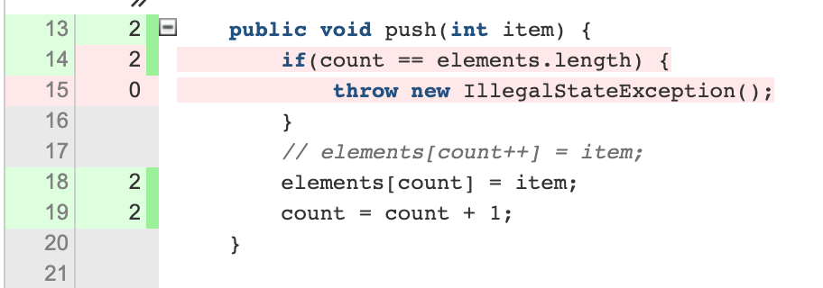
Code coverage has been widely adopted by software companies. Google, for example, has its own guidelines when interpreting and using code coverage. They can be consulted for more details in (64) and (65). In these guidelines, Google developers express that there is no “ideal code coverage number” that can be applied to all software products. The coverage level depends on the relevance of the code, how often a code location changes and how long is the code expected to be used. In broad terms they consider a 60% coverage as acceptable, 75% as commendable and 90% as exemplary. They argue that developers should aim at improving code coverage, but the effort should be directed to improve badly covered code, for example to go from 30% to 70% instead of going from 90% to 95% in a project. Raising an already very high code coverage may require a lot of effort with little gain. Coverage metrics are used inside the company together with static analysis to support code reviews.
These practices are not exclusive of big companies like Google. The XWiki Project\footnote{http://www.xwiki.org/} builds a Java platform to develop collaborative applications. The contributors of this project pay close attention to the quality of their test suite and have incorporated coverage monitoring into their development practices. The main XWiki codebase is composed by 3 Maven multi-module projects with more than 40 submodules each. These modules may contain more than 30K lines of application code and more than 9K of test code implementing several thousands of test cases. The entire development process is monitored in a CI server running Jenkins.
The build pipeline in the CI includes actions to check the quality of the code and tests. In particular, they monitor the coverage achieved by the test suite. Each module in the codebase has a predefined threshold and the code coverage can not decrease below this value, otherwise the build will fail. In this way, if a developer adds some code she has to also provide new tests cases so the coverage ratio remains above or equal the predefined value. If a developer achieves a coverage above threshold, then she is given the possibility to raise the value for the module. In this way it is ensured that the code coverage never decreases. This is what they call the Ratchet Effect. This strategy has led to an effective use of the code coverage metric and a substantial increment on coverage levels (66).
Mutation testing has not gained an adoption as broad as code coverage has. The mutation analysis provides a better criterion for the quality of the tests but it is a complex and expensive process, sometimes hard to interpret. In terms of tooling, there are a few options available. Among them, the most popular alternative is PIT or PITest. PIT instruments mutants in the compiled bytecode and integrates with all major build systems like Ant, Gradle and Maven. Other tools for Java include Javalanche which also manipulates bytecode to inject faults and Major that operates at the source code level. Major is integrated with the Java compiler and provides a mechanism to define new mutation operators.
PIT was develop for industry use unlike many other tools that have been developed mainly for research purposes. Apart for a good integration with most build systems, the tool has a pluggable architecture allowing its configuration and extension. The implements many of the traditional mutation operators like: changing instances of comparison operators, arithmetic operators, removing method invocations, perturbing method results and many others. PIT also implements many strategies to make mutation testing affordable. For example it creates mutants in memory from the compiled code and not the source code. It computes code coverage before running the analysis, so only mutants reached by test cases are inspected and only the test cases reaching each mutant are executed. The test cases are also prioritized, so faster test cases are executed first.
Mutation testing has gained some traction in the last few years. Companies like Google have started using it. Petrovic and Ivankovic (67) have described how the company uses mutation analysis in their codebase. They explain that the Google repository contains about two billion lines of code and on average, 40000 changes are incorporated every workday and 60\% of them are created by automated systems. In this environment it is not practical to compute a mutation score for the entire codebase, and it is very hard to provide an actionable feedback to developers
Most changes to the code pass through a code review process. So, the mutation testing feedback is incorporated into code reviews along with static analysis and code coverage. This eliminates the need for developers to run a separated program and act upon its output. To make the mutation analysis feasible the system shows at most one mutant by covered line. To further reduce the number of mutants, they classify each node of the Abstract Syntax Tree (AST) as important or non-important. To do this, they maintain a curated collection of simple AST nodes classified by experts. The system keeps updating this database with the feedback from the reviewing process. This selection may suppress relevant live mutants but there is a good tradeoff between correctness and usability as as the number of potential mutants is always much larger than what can be presented to reviewers.
The system analyses programs written in C++, Java, Python, Go, JavaScript, TypeScript and Common Lisp. It has been validated with more than 1M mutants in more than 70K diffs. 150K live mutants were presented and 11K received feedback. 75% of the findings with feedback were reported to be useful for test improvement. The company has also noticed differences related to the survival ratio of mutants when contrasted with the programming language and mutation operator.
3.4.3. Test doubles
Often, code units depend on other software components to achieve their functionalities. When testing a unit it may happen that some of its dependencies are not yet implemented and we only have an interface. It could also happen that these dependencies perform actions that can’t be undone, like sending an email to a customer which makes them not suited for testing. In such scenarios we use test doubles. Doubles as in stunt doubles.
Ammann and Offutt (4) define test doubles as software components implementing only partial functionalities that are used during testing in place of actual production components. That is, we create classes that do not contain the actual functionality but provide a minimal working code that we can leverage in our tests.
Let’s illustrate test doubles with a simplified example. Suppose we are building an e-commerce website. In our code (Listing 63) we have notions about customers, products and shopping carts. A product has a base price. A shopping cart belongs to a user and contains a collection of products. This class uses a service PromoService to obtain the active promotions for a user. A promotion applies to a product and informs the net discount for a product with getDisscountFor. A shopping cart computes the final price of the collection of products using the active promotions and applies all discounts.
class User {
    ...
}

class Product {
    ...

    public BigDecimal getBasePrice() {
        ...
    }
}

class ShoppingCart {

    User user;
    Collection<Product> products;
    PromoService service;

    public BigDecimal getTotalBasePrice() {
        // Sum of all base prices
        ...
    }

    public BigDecimal getFinalPrice() {
        // Uses PromoService to obtain the active propomotions for the user
        // Computes the final price of each product by using the disccounts
        ...
    }

}

interface PromoService {

    Collection<Promotion> getActivePromotions(User user);

}

interface Promotion {

    boolean appliesTo(Product product);

    BigDecimal getDiscountFor(Product product);

}
Suppose we are given the task to test getFinalPrice. ShoppingCart depends on PromoService. The actual implementation of this interface could be still under development at the moment we will test ShoppingCart. It could also be the case, that the actual implementation requires access to a database which might make the test slower. To avoid dealing with these issues we can create test doubles for PromoService.
For example, one scenario we would like to test is when the user has no active promotions. Instead of messing with the actual production code, we can create a simple test double like in Listing 64. This double returns a predefined constant value. Such test doubles are usually called stubs. Apart from returning fixed values, stubs could also return values selected from a collection, or values that depend on the input or even random values.
PromoService to test the scenario where the user has no active promotions and an extract of a test case using the test double.
class NoPromoServiceStub implements PromoService {
    public Collection<Promotion> getActivePromotions(User user) {
        return Collections.empty();
    }
}

...

@Test
public void testPriceNoActivePromotion() {
    ShoppingCart cart = ...
    cart.setPromoService(new NoPromoServiceStub());

    assertEquals(cart.getTotalBasePrice(), cart.getFinalPrice(),
                "With no promotions the final price must be equal to the total base price");
}
Since we are testing the interaction between software components, sometimes it is useful to add verifications inside the code of a test double. This could help us verify, for example, that a method has been called a certain number of times. In our example, we could verify that getActivePromotions is invoked only once. Test doubles implementing verifications on the interaction of components are usually called mocks.
| Some authors state that mocks are a kind of specialized stubs. As Ammann and Offutt say, whether a mock is also a stub is not relevant for practical purposes. Other authors may include more classifications for test doubles such as: dummies, spies and fakes, depending on the amount of functionality they implement. |
Test doubles have several advantages in practice. We already discussed that test doubles are helpful when a component has not been implemented to create test cases matching the specification. Then, the implementation can leverage these early tests and the development of other functionalities is not blocked. As we discussed before, test doubles also avoid the execution during testing of actions that are permanent or hard to undone, like writing to a database or sending an email. Test doubles also provide a nice sandbox when dealing with external components that may not always be available or their execution takes a lot of time, for example, using a remote REST API. In such scenarios, using test doubles guarantee that our test cases will remain fast and will not fail if the service is not available.
We can choose to create test doubles manually, like we did before with the stub. In such a simple example manually creating the stub was enough. But, for more complex scenarios and to perform more complex verifications inside mocks we might better use available mocking frameworks.
Mocking frameworks: Mockito
Our tests should be simple to understand, as we need to map them to the specification and we need to maintain them. Creating test doubles by hand could make our test cases more complex. Mocking frameworks are software tools that keep the creation of test doubles clean and easy to incorporate to our test code. One of such frameworks for Java is Mockito
Mockito has an easy to use and understand fluent API. With it we can create and verify stubs and mocks almost declaratively. Listing 65 shows an example of who to rewrite Listing 64 with Mockito.
@Test
public void testPriceNoActivePromotion() {

    PromoService service = mock(PromoService.class); (1)

    when(service.getActivePromotionsFor(any())) (2)
        .thenReturn(Collections.emptyList());

    ShoppingCart cart = ...
    cart.setPromoService(service);

    assertEquals(cart.getTotalBasePrice(), cart.getFinalPrice(),
                "With no promotions the final price must be equal to the total base price");
}| 1 | Instructs Mockito to create a test double for PromoService. |
| 2 | Specifies the behavior on getActivePromotionsFor. The double is instructed to return an empty list for any argument. |
Listing 66 shows an extract of a test case verifying that getFinalPrice invokes getActivePromotionsFor only once. If during the execution of the test case, the method is not invoked or it is invoked two or more times, the test case will fail.
@Test
public void testPromotionsConsutledOnce() {
    PromoService service = mock(PromoService.class);
    ShoppingCart cart = ...
    cart.setPromoService(service)
    BigDecimal finalPrice = cart.getFinalPrice();

    ...

    verify(service, times(1)).getActivePromotionsFor(any()); (1)
}| 1 | Assertion to verify the number of times the method was invoked. |
In both examples Mockito prevented the manual creation of classes and provided an easy to understand mechanism to incorporate the test doubles. The test code remains simple and self-contained. Also, the same general mechanism can be used for all our classes. The framework also allows mocking concrete classes beyond only interfaces. It also provides ways to verify that a method was invoked with specific arguments, and even to still invoke concrete methods while observing their behavior.
Best practices and misuses
Test doubles are powerful allies for testing, but they can be often misused. There are even testing smells that concern only mocks and stubs.
One of the test smells coined for mocks is the Mock Happy smell. It refers to test cases that require many mocks to run. These test cases are often fragile and hard to understand (53) and maintain.
In general terms, the overuse of mocks can damage the quality of our test code. For example, we should avoid mocking value types or any other immutable type or any class that is simple enough to control and observe. Mocking those classes may result in a test code that brings little value and it may even be harder to understand than using the original class directly.
We should avoid mocking third party classes as much as possible. When we mock a class we make assumptions on their behavior. Those assumptions may be wrong if we don’t fully understand how external classes behave in all scenarios. We should create mocks mostly for our own code. Expressing an incorrect behavior of external dependencies with mocks leads to test cases that do not fail, yet, the code will break in production (68).
3.5. The role of testability
High quality test cases are concise, clear, repeatable, independent, efficient and maintainable (54). A good test suite facilitates the development of our product as it catches bugs earlier. However, code quality has also an important effect over the quality of the test cases. Low quality code is hard to test. If the classes in the code are tightly coupled, or the software has hidden external dependencies, or if it forcibly depends on external services, then it is hard for test cases to instantiate the components and set them in the specific states required for testing (69).
Therefore, we should design software with tests in mind, that is, we should design software to be testable. Testability is the property of a system that characterizes how easy it is to test. It can be defined in terms of two other sub-properties: controllability: how easy it is so set a software component in the desired state and, observability: how easy it is to observe and verify the state of the component. In other words, a software is testable if its state is easy to control an observe. High quality code leads to a highly testable software.
For example, loosely coupled classes with high cohesion, that observe the Single Responsibility Principle are easier to instantiate and also lead to easier and more understandable test cases. Complex code will necessary produce complex and hard to understand test cases. Coupled classes will also make the test code unnecessarily large and harder to read since we will need to create many objects at the same time to test one of them.
These symptoms of bad code often manifest themselves during testing. In most occasions it is better to go back and redesign our software components than creating complex test cases. For example repeating the same mocking setup across many test cases might be a signal of tight coupling that should be better solved in the application code than making the test code repetitive (70).
Design patterns are general solutions to recurring problems in programming (72). These solutions are proven to be effective and, if well used, they help making the code easier to understand. The good application of design patterns also make the code more testable (69), (71). Two patterns often used as examples of testing facilitators and in particular to make mocking easier are Dependency Injection and Repository.
Using Dependency Injection, classes receive their dependencies instead of explicitly creating them. Classes then depend on abstractions, interfaces, that can be easily exchanged. Also, since classes are not in charge of creating their dependencies their code is simpler. Our example with PromoService is loosely based in this design pattern. This pattern makes it extremely easy to exchange the dependency, which is helpful for mocking and stubbing as we saw in the example. It also makes the component more controllable as we can create dependencies more easily than production code.
With the Repository pattern we create a class that manages all access to the data. This class encapsulates and hides the actual data access operations, separating even more our components from the data access implementation and the concrete storage method used in production. Using this design pattern facilitates mocking the data access mechanisms which in turn facilitates the verification of how our code interacts with the data components. We also avoid making actual database modifications that we might need to undo to keep our tests repeatable.
3.6. Test Driven Development
Test Driven Development (TDD) is an approach to software development that encourages writing tests first, before writing any application code. The concepts behind TDD are derived from the Extreme Programming movement in the late 90’s. The popularization of this methodology is credited to Kent Beck, who also created SUnit, a unit testing framework for Smalltalk and inceptor of the entire xUnit framework family. Beck also participated in the development of JUnit together with Erich Gamma.
In his seminal book, Test-driven development: by example (73) Beck states that TDD follows two simple rules:
-
Don’t write a line of new code unless you first have a failing automated test.
-
Eliminate duplication.
These two rules induce the organization of programming tasks in a cycle, known as the Red/Green/Refactor cycle:
- Red
-
Write a simple and short test that does not work. Since the application code isn’t already entirely written, the test might not even compile. The name of this phase makes allusion to the fact that failing tests are usually shown in red in many programming environments.
- Green
-
Take any quick coding action required to make the failing test work. In this phase we will introduce low quality code with repetitions and non-optimal solutions. Our only goal is to make the test pass, hence the Green name.
- Refactor
-
Eliminate any redundancy or duplication and improve the code added to make the test pass by refactoring. This refactoring benefits for the previously created tests. If we make a mistake during this phase, the tests in place will catch it early enough.
If we use TDD, whenever we add a new feature to our product we must start this cycle. At the end of each phase of the cycle we must execute all tests that have been created and not only the one we just added. In the Red phase only the new test should fail for the expected reasons. If the test does not fail, then it is wrong or does not bring any value to the test suite. No other test should fail by the addition of this new test. After the Green phase all tests must pass. The new code should not brake any existing test and it must be created to make the new test pass. During the Refactoring phase the test suite becomes a safety net in which we can rely to improve the quality of our code without introducing changes that break the expected behavior.
TDD requires an efficient test suite that can be executed regularly to obtain early feedback from tests. It also requires developers to write their own test cases. These premises are actually at the core of modern software development.
The methodology has true practical advantages (71). On the one hand, it forces the creation of tests that might otherwise never been written. On the other hand, the application code is designed from the users' perspective and it enforces developers to write testable application code. The effective use of TDD shall produce in the long term code with fewer bugs and shall reduce the need for debugging as tests should be informative enough to diagnose any fault.
Like any other methodology TDD has gained adepts and detractors which regularly engage in never-ending discussions. Both sides use strong arguments to make their cases. However, we must keep in mind that, again, as any practical approach, TDD fits better the practices of ones and not the ways of others. We should not use it blindly and we should think whether its application may bring more damage than good.
Applying TDD does not mean that we don’t need a careful design of our product. An initial and comprehensive design phase is crucial for the quality of our software (74). A good design actually facilitates the application of TDD, as it helps keeping the tests focused. But it is not true in the opposite sense. Without a clear design, we will be making the design on the fly and TDD may lead to bad design choices.
Real life is not the same as the small and carefully crafted examples, often used to introduce TDD. In those examples, the requirements are clear and will not change. However, in a real development projects the requirements may change in time and are often vague. We should take that into account otherwise we will find ourselves adapting our code and our prematurely created tests many times increasing the cost of maintenance and development (75).
TDD favors a strong focus on unit testing. Over-specifying our code with unit tests may lead to unuseful test cases that may well verify assertions that under no circumstances will be false. It may also lead to an important amount of tests for very simple code. It may also induce to the overuse of mocks, whose perils we already discussed in the previous section. In practice, there are scenarios when a couple of higher level tests can be more useful than tens of unit tests. This tradeoff should be carefully taken into account (76).
Projects with well defined functional requirements unlikely to change much seem to be a good match for TDD. Take as example the creation of a compiler. The specification of the source and target language do not change much in time. The structure of the tests is also well define in the for of input and expected output. In such a project we will be creating tests cases directly matching the specification and main goal of the product.
Maybe, as Eric Gunnerson puts it, the most relevant phase of TDD is not creating the tests but the regular code refactoring. Refactoring should lead to a better designed product with high quality code, with low coupling and better testability (77).
But, should we use TDD or not? There is no simple answer. We must use the approach that better fits our practices. In the words of Martin Fowler (78):
Everything still boils down to the point that if you’re involved in software development you have to be thoughtful about it, you have to build up what practices work for you and your team, you can’t take any technique blindly. You need to try it, use it, overuse it, and find what works for you and your team. We’re not in a codified science, so we have to work with our own experience.
Is TDD Dead?
4. Fuzzing
| This section follows the structure of the Lexical Fuzzing chapter from The Fuzzing Book. It also replicates part of the experiments from this book using a different tools. The supporting code can be checked at https://github.com/oscarlvp/simplefuzzing |
Last section discussed the main ideas behind software testing. There, we explored the best testing practices and the advantages of automated test execution. However, not only test execution can be automated. It is also possible to automatically create test cases.
Fuzzing is one of the most successful techniques exploited in practice to generate test cases and discover program failures. It is a sort of real-life comic book hero with a cool origin story humble beginnings an it is literarily saving the world today.
The main idea behind fuzzing is simple: we generate random inputs and then check if the execution of the program fails or crashes while using those inputs.
According to The Fuzzing Book (79), fuzzing was born in the late 1980’s when professor Barton Miller from the University of Wisconsin-Madison was connected to his workstation via a telephone line. There was a thunderstorm that caused noise in the line, which, in turn, caused the terminal commands get random inputs. The programs he was using crashed continuously. This inspired him to study the robustness of programs against random inputs. So, professor Miller wrote an assignment for his students asking them to create a fuzz generator (fuzzer). The generator should produce random character streams that students should use as input of UNIX utilities to find failures, that is, to break them. With this naive technique, Miller and his students were able to find actual failures and bugs in well tested utilities like vi and emacs. Since then, fuzzing has become a mainstream technique to test programs. Even if it took a while for the scientific community to accept the effectiveness of such a simple technique, a lot of research has been invested on improving fuzzing and several industry-level fuzzers have been developed through the years.
| Coming from a country where we still use the telephone line to connect to the Internet I find this fuzzing origin story quite amusing. First, I’m surprised to know how reliable professor Miller’s telephone line was in regular days. Mine is always noisy. Second, I consider a thunderstorm a red alert situation requiring instant and total disconnection to avoid my modem getting fried. Anyways, this cool short story gave us one of the coolest testing techniques, that boldly took us where no tester has gone before. |
Listing 67 shows a pseudo-code outline of a simple fuzzing algorithm.
input: program
output: failures // Failure inducing inputs
procedure:
until stopping conditions:
    input = generate random input
    failure = execute program with input
    if failure:
        add (input, failure) to failures
return failures
From this pseudo-code we may identify three subproblems whose solutions directly affect the effectiveness of a fuzzing process: what to observe during the program execution, how to generate the inputs and when to stop fuzzing the program. Not by chance, these questions are closely related to the problems we identified from [testing-process] when discussing the general testing process. Fuzzing can be seen as a fully automated instance of this general process.
The answer to the third question might be a matter of resources. The longer we let a fuzzer run the higher the chances it has to discover new execution paths and faults. But, a fuzzer can not run forever. Commonly, we stop fuzzing a program after the first failure has been detected or after a certain amount of hours. This time depends on our infrastructure and even the program under test. It makes no sense to fuzz a small program for a whole week. We may also stop fuzzing after a certain number of generated inputs or a certain number of program executions, that can be limited by our budget if we run the fuzzer in the cloud. It is also possible to rely on theoretical statistical results to estimate the likelihood with which a fuzzer may discover new execution paths and assess how well it is performing in that sense. A nice overview on this particular idea can be found in the corresponding chapter When to Stop Fuzzing of The Fuzzing Book (79).
4.1. What to observe?
Fault triggering inputs are detected by observing the execution of the program under test. Observing different program properties enables the discovery of different types of program faults.
The first obvious observation we can make is to check whether a program terminates abruptly or crashes with a given input. A program crash indicates the presence of a fault.
A crash may occur when the program under test throws an unhandled exception. In POSIX systems, some unhandled signals as SIGILL (invalid instruction), SIGSEGV (segmentation fault) and SIGABRT (execution aborted) also produce an abnormal program termination.
There may be many reason behind a program crash, for example, a program may: * try to execute actions without having the right privileges: accessing to a restricted file, the camera or any other resource. * try to write or read outside the assigned memory location. This is known as a segmentation fault. IN POSIX systems this program receives a SIGSEGV signal. In Windows it gets an access violation exception. * pass the wrong parameters to a machine instruction or to a function which may end, for example, in a division by zero. * abort the execution due an invalid internal state that produces an assertion failure.
Some programs do not check the boundaries of the memory buffers they modify. These programs may corrupt the memory adjacent to the buffer. This is known as a buffer overflow. Buffer overflows may cause the aforementioned segmentation faults. However, not all overflows cause a program crash and many of them become vulnerabilities that can be exploited to execute non-authorized code or to leak unwanted information like the Heartbleed bug we saw in Figure 2. Actually, the Heartbleed vulnerability was discovered with the help of fuzzing.
Some compilers, such as Clang, are able to instrument the compiled code of a program to include memory error checks and signal the occurrence of buffer overflows. These instrumented programs can be fuzzed to find this type of fault. Other similar instrumentations can be used to spot uninitialized memory accesses, type conversions and numeric operations that may end in overflows and even concurrent actions that may end in race conditions.
In the last section we used assertions to verify the state of a program after the execution of a test case. In fuzzing we use randomly generated inputs. Therefore, it is hard to create an assertion with the expected program result for each input. However, we can use assertions to verify invariants, that is, properties the output of a program must meet no matter the input. This is known as property testing.
Suppose we have a function that computes the height of a given tree. For any tree the height must be greater or equal to zero. To test this function, using property testing, we can generate random tree instances and check that all heights are non-negative. In other contexts we could verify, for example, that all resources has been closed after processing a sequence of random inputs.
There are many good libraries implementing property testing and we shall discuss them in a later section. However, this approach is not hard to implement using built-in JUnit functionalities. Listing 68 shows a general template that can be used for that.
@TestFactory (1)
Stream<DynamicTest> checkProperty() {
    Iterator<TInput> inputs = ...; (2)
    Function<TInput, String> name = ...; (3)
    Predicate<TInput> property = ...; (4)
    ThrowingConsumer<TInput> verification = input -> assertTrue(property.test(input)); (5)
    return DynamicTest.stream(inputs, name, verification); (6)
}| 1 | The @TestFactory annotation marks a method as a producer of test cases. The method should return a collection or a stream of DynamicTest instances. Each test instance is considered as an independent test case. |
| 2 | Here we implement the input generation as an Iterator. The iterator should return random input values. |
| 3 | Each test case in JUnit should have a name. Here we use a function to generate string representation for each input value. This name can not be null or blank. |
| 4 | The property to verify is implemented as a predicate that must return true for every input. |
| 5 | This is the actual verification that each test case shall perform. It simply uses assertTrue to check that the property is true. |
| 6 | Returns the stream of DynamicTest instances. |
Using @TestFactory each test case is executed independently and even in parallel. At the end of the test case stream JUnit reports all failing inputs.
Provided we have a tree generator, we could implement the tree height verification as shown in Listing 69.
@TestFactory
Stream<DynamicTest> checkProperty() {
    return DynamicTest.stream(
            getTreeGenerator(),
            Tree::toString,
            tree -> assertTrue(tree.height() >= 0)
    );
}
Property verification is simple. Generating interesting inputs remains the hardest part, as in all fuzzing approaches.
A scenario that is particularly well suited for property testing and fuzzing appears when we must implement a pair of encoding, decoding functions. An encoding function takes a value from domain A and transforms it into a value of domain B. The decoding function takes a value from B and produces a value from A. In many cases, we can pass the result of the encoding function as input to the decoding function and obtain the initial input. Using this property we can verify at the same time both, the encoding and the decoding functions.
Consider an example in which we are implementing two pairs of functions: encodeBase64 that takes an array of bytes and obtains a string in base 64 representing the array and decodeBase64, implementing the opposite functionality, it takes an string in base 64 and produces the corresponding byte array. We can verify both functions by generating a random byte array, encoding it into a string, then decoding the string and verify that the final result is equal to the input.
This example could be implemented as shown in Listing 70.
@TestFactory
Stream<DynamicTest> checkProperty() {
    Iterator<byte[]> generator = getByteArrayGenerator();
    return DynamicTest.stream(generator, Arrays::toString,
            array -> {
                assertArrayEquals(array, decodeBase64(encodeBase64(array)));
            });
}
Sometimes we have a reference implementation of the functionality we are building. This may happen, or example, when we are migrating a dependency of our program from one version to another, or when we are porting an already existing functionality to another programming language or framework. If those changes are not supposed to affect the output of the program under test, we can verify the new implementation by comparing the output to the result produced by the reference implementation. In such scenario we can generate random inputs and assert that both results are equal as shown in Listing 71.
@TestFactory
Stream<DynamicTest> checkProperty() {
    return DynamicTest.stream(getInputGenerator(), PropertyTesting::name,
            input -> assertEquals(reference(input), implementation(input))
    );
}
We can also use automatically generated inputs to test at the same time multiple programs with the same functionality. Any difference in their behavior or result with these random inputs may indicate the presence of faults. This is known as differential fuzzing or differential testing and has been very successful at discovering program vulnerabilities (80) (81).
4.2. How to generate random inputs?
An effective fuzzing strategy generates random inputs able to discover faults. This is arguably the hardest challenge for fuzzing. Recalling the RIPR model, the generated inputs should be able to reach the faults, infect the program state and propagate the effects of the fault to the output of the program. Therefore, the generated inputs should be able to produce as many executions paths as possible and reach as much program instructions and branches as possible.
American Fuzzy Lop (AFL), one of the most used fuzzers, focuses on reaching as much program branches as it can. Its authors claim that branch coverage provides more insight on the execution path than block coverage (82). Two execution paths may have the same block or statement coverage, but different branch coverage. Branch coverage can discover faults in conditions that become noticeable through wrong control changes. The AFL authors explain that security vulnerabilities are often associated with these incorrect program state transitions.
The simplest approach to generate program inputs might be to randomly generate from scratch any value in the input domain. This could be fairly easy if the inputs consists on numeric values and byte arrays or strings with no format.
However, this approach is quite limited when trying to test programs expecting structured inputs. In programs that process images, JSON files, or strings with a syntactic structure like an expression or code, it is really hard to achieve a high statement or branch coverage using only random inputs generated from scratch. These generated inputs can help test the program against unexpected values but, in many cases, faults can appear after parts of the input has been processed. That is, when the input contains correct and incorrect fragments at the same time.
Structured inputs are commonly composed by keywords or recurrent fragments. For example, HTML documents are composed by tags such as <a>, </a>, <i>, program code contain keywords and literals or a configuration file contains the name of the configuration options. A way to increase the chances to generate inputs able to cover more branches is to use a dictionary containing those keywords. We can generate better inputs by randomly combining these keywords or terms. These terms can be manually selected or even extracted from the code of the program under test.
Suppose we have created an ExpressionParser class that implements a recursive descent parser for simple arithmetic expressions that may contain the usual arithmetic operators +, -, *, /, negation, parenthesis, usual floating point literals, references to predefined constants such as PI or E and invocations to predefined functions such as min, exp, log and alike. The parser can be used as shown in Listing 72. For a given string, the parser produces an Expression containing an abstract syntax tree of the given input. If the input is incorrect, the parser throws a ParseException.
try {
    ExpressionParser parser = new ExpressionParser();
    Expression exp = parser.parse("2 * - (1 + sin(PI))")
    System.out.println(exp.evaluate());
} catch(ParseException exc) {
    System.out.println("Incorrect input");
}
We can try the input generation strategies on this class to evaluate their performance according to the number of branches they can reach and to check if we can find any unexpected error (other than a ParseException) like NullPointerException.
To generate strings we pick a random sequence of characters from the following predefined alphabet: ` \tabcdefghijklmnopqrstuvwxyzABCDEFGHIJKLMNOPQRSTUVWXYZ0123456789+-*/(),.!@;[]{}`. This alphabet contains whitespaces, letters, numbers and symbols that can be used to conform valid expressions, but it also contains invalid symbols according to the parser specification such as !@;[]{}. Each generated string has a random length between 0 and 100. Here are samples of the strings that can be generated in this way:
-
q]Mwd7)9.f-5A}E -
HI- q1H2Cs}r9KTmOeqBu/rO+V7VG]s[B[ -
i.U07X)XAKJI2VTVn)qbqhHQ5X30kk 5j;2mlrbVow[(HCEblAsMVe9K CGq9Fg@)93eUho9JTUxU -
{D@ -
;!/hQW/c3nmS 0UGj4kWIJQ{2Gjb.Jlx)BeWz. Ay.]RO mrH!GICyVR
Notice how they do not resemble valid expression. It is extremely hard to get a string close to be a valid expression with pure random character selection.
To generate inputs using a dictionary of terms we can use the following keywords: "pow", , `"min", `"sin", `"cos", `"1", `".5", `"1e-5", `"(", `")", `"+", `"-", `"*", `"/", `"PI", `"E"`" ". These keywords contain whitespaces, valid function and constant identifiers, valid literals and valid symbols. To create an input we randomly select between 0 and 10 of these terms, with possible repetitions. The dictionary approach is not exactly very advantageous in this example. It would suite better in actual code, such as SQL queries where it has been shown to be quite efficient (83). While still random, the inputs generated this way are closer to a valid expression:
-
/- -
1 -
cospow++E+1e-5+min -
( PIE1/( -
//pow.5pow(-pow -
+1e-5 powpowcos
To compare the performance of these two strategies we replicate the experiment model from The Fuzzing Book. We fuzz the ExpressionParser with different numbers of generated inputs from 1 to 100. For each input, we execute each fuzzing strategy 30 times and compute the average number of branches reached using the generated inputs. This shall tell us what is the expected number of branches for a given number of inputs that each strategy can reach. Figure 17 shows the result of this experiment.
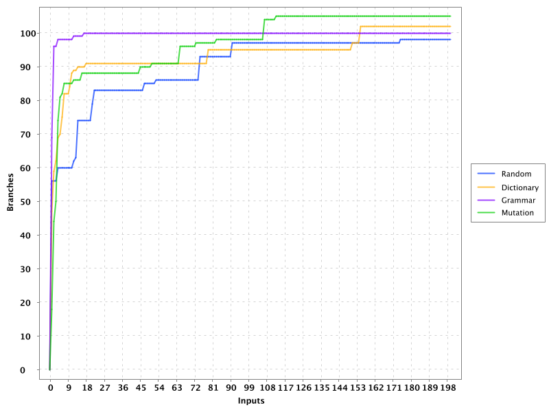
The plots shows that, when generating only 9 inputs, the random string approach (Random series in the plot) reaches 60 branches on average, while the dictionary based generation reaches more than 80 branches. As we increase the number of inputs both approaches discover more branches, but the dictionary based generation requires less inputs in general to discover more branches.
In most cases the structure of valid inputs can be expressed through finite automata or their equivalent regular expressions or with formal grammars. These formalism can be leveraged to quickly generate a large sets of valid inputs. The efficient generation of strings from formal grammars has its own practical challenges. The topic is largely discussed in the Syntactical Fuzzing chapter of The Fuzing Book (79). Using grammars to create valid inputs help us to rapidly reach more branches than with random inputs. However, these valid inputs are often closer to the happy path than corner cases where most faults arise.
Valid inputs for our ExpressionParser can be generated using the following context free grammar:
expression = term, { ( "+" | "-" ), term } ;

term = factor, { ("*" | "/"), factor } ;

factor = "-", atom ;

atom = number | identifier | invocation | "(", expression, ")" ;

invocation = identifier, "(" [ arguments ] ")" ;

arguments = expression, { "," expresssion } ;

identifier = letter, { letter | digit } ;

digits = digit, { digit } ;

number = (  digits, [ ".", digits ] ), [ "e", ["-"], digits ] ;

letter = "A" | "B" | "C" | "D" | "E" | "F" | "G"
       | "H" | "I" | "J" | "K" | "L" | "M" | "N"
       | "O" | "P" | "Q" | "R" | "S" | "T" | "U"
       | "V" | "W" | "X" | "Y" | "Z" | "a" | "b"
       | "c" | "d" | "e" | "f" | "g" | "h" | "i"
       | "j" | "k" | "l" | "m" | "n" | "o" | "p"
       | "q" | "r" | "s" | "t" | "u" | "v" | "w"
       | "x" | "y" | "z" ;

digit = "0" | "1" | "2" | "3" | "4" | "5" | "6" | "7" | "8" | "9" ;| We used Extended Backus–Naur form to write the grammar and we omitted the whitespace sequences for readability. |
With the help of this grammar we can generate inputs such as:
-
R * 9 + 4 - 9 -
X - -i * (1) + 4 -
1 * 2 + e * x -
(I * 4 / R / (H)) -
(I(8, 3) * (u - -b))
In Figure 17 the series named Grammar shows the results of fuzzing ExpressionParser with inputs generated with this grammar. It can be noticed that these inputs quickly reach a high number branches but do not make any progress beyond that. All generated inputs are syntactically valid, therefore this generation strategy never reaches branches executed for invalid inputs.
Mutation based fuzzing proposes to use valid inputs in a different way. This approach uses a set of valid inputs as initial seeds. These inputs may be generated with the help of a grammar, or they can be manually specified. They are first used to execute the program. Then to generate a new input, we randomly pick one of the seeds and we mutate it. That is, we perform a small modification on the seed to create a new input. Listing 74 shows the pseudo-code of this strategy.
input: program, seeds
output: failures
procedure:

for seed in seeds:
    failure = execute program with seed
    if failure:
        add (seed, failure) to failures

until stopping conditions:
    take seed from seeds
    input = mutate seed
    failure = execute program with input
    if failure:
        add (input, failure) to failures
return failures
Mutations (not to confuse them with the mutation from mutation testing) can be very simple changes. For example, if the input is a string, we can mutate the seed by inserting a random character at a random position, or removing a random character or even removing a random slice of the string. We could also use a dictionary to insert a random keyword in a random position of the input. It may also make sense to perform more than one mutation at once on the same seed to increase the difference between the seed and the new input.
For our example, we use a mutation based fuzzer with the following seeds " ", "1", "1 + 2", "min(1, 2)", "-1". As mutations we use the following:
- remove a random character from the seed.
- add a random character from the alphabet we used in our first fuzzer in a random position
- replace a random character from the seed with another random character from the same alphabet
For each seed we perform between 2 and 5 random mutations. This produces inputs like the following:
-
1 + -
9 mp(1, 2) -
min(12) -
m,n( 2) -
+d2E -
P-M{R -
1 + 2H -
n(1,82) -
*in,O)
The results of the mutation based fuzzing strategy can be seen in the Mutation series shown in Figure 17. Notice how this strategy reaches the highest number of branches and even converges faster to the final results.
The effectiveness of mutation based fuzzing depends on the initial seed selection and the nature of the mutations. In our example, including seeds with more arithmetic operators and even combinations on the operators might make the strategy discover more branches.
The input generation strategies discussed so far do not rely on any information about the internal structure of the program under test or the program execution to generate a new input. This is known as black box fuzzing. However, monitoring the program execution can lead to valuable information for the generation process. We can for, example, exploit more the inputs that execute hard-to-reach branches using them as seeds.
Greybox fuzzing observes partial information from the program execution. For example, it can collect the branches executed with each input. This information can be used to affect the input generation. We can extend the mutation based fuzzing approach by augmenting the seeds with inputs that reach new branches. This approach is outlined in Listing 75. The rationale behind this idea is that mutating inputs reaching new branches increases the chances to discover new execution paths.
input: program, seeds
output: failures
procedure:

covered_branches = {}

for seed in seeds:
    failure, path = execute program with seed
    if failure:
        add (seed, failure) to failures
    else:
        add all branches in path to covered_branches

pool = [...seeds]
until stopping conditions:
    take seed from pool
    input = mutate seed
    failure, path = execute program with input
    if failure:
        add (input, failure) to failures
    else:
        if exists branch in path not in covered_branches:
            add all branches in path to covered_branches
            add input to pool
return failures
In both, the approach above and the initial mutation based approach, all seeds are selected with the same probability to generate a new input. We can extend the original idea to favor the selection of more desirable seeds, for example, those producing less frequent execution paths. This new approach should help the fuzzing process cover more program elements in less time. It uses a power schedule assigning an energy value to each seed. The energy is the likelihood of a seed to be selected. The concrete energy assigned to each input depends on the characteristics we want to explore with seeds. Its value could be, for instance, inversely proportional to the number of times the same path has been executed, if we want to favor seeds with least explored program locations. It could also depend on the size of the seed or the number of branches covered in the execution. The overall process remains the same, the only thing that changes in this new approach with respect to greybox fuzzing is that each seed is selected according to the probability distribution defined by the energy of the seeds.
Both, the greybox strategy shown in Listing 75 and the strategy using power schedules should lead to a faster branch discovery than the initial mutation based fuzzing. To compare them, we replicate the previous experiment. This time we use as seed a single empty string and the same mutations as before in all three fuzzing approaches. Since the initial seed is reduced we extend the number of inputs until 1000. The results are shown in Figure 18.
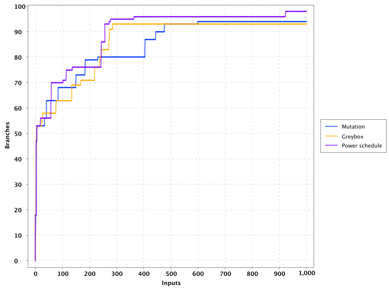
Notice in the plot how the approach using power schedules is faster at discovering new branches and obtains the higher number in the end. In our example, both the blackbox mutation based fuzzer and the greybox fuzzer have comparable results with the latter reaching branches faster at some moments.
4.3. Libraries, tools and practice
Fuzzing has become a mainstream testing technique. It has shown to be really effective in practice, in particular, to detect security issues in real software. One of the most used fuzzers is the already mentioned American Fuzzy Lop (AFL), a fuzzer for compiled C programs.
Roughly speaking, AFL takes an initial collection of user-provided files as seeds. New inputs are generated by subsequently mutating these seeds. First it applies simpler, deterministic and almost exhaustive mutations, like sequentially flipping from one to four bits in a row for the entire seed to generate several new inputs or replacing parts of the seed with predefined integer values, known to cause troubles like -1 MAX_INT-1 and so on. Then, it applies random mutations that could be the deletion, insertion or replacement of parts of the seed. The tool keeps track of the branch coverage for each input. The initial set of seeds is augmented with those inputs that reach new branches. Inputs are actually processed in a queue that gives priority to smaller files. Inputs for which the program under test crashes are reported at the end along with the set of all inputs reaching new branches.
AFL has been able to discover a large number of faults and security vulnerabilities in real life, well tested and widely used software like ImageMagick, gcc, qemu, git, OpenSSL, sqlite and many others.
The success of the tool has originated many derived projects and extensions to other languages like go-fuzz for Go, python-afl for Python, libFuzzer for LLVM and the Kelinci project which implements a Java interface for AFL.
On its side, property based testing has been popularized among developers through libraries like QuickCheck for Haskell and its many derivate projects. Among the most popular alternatives for Java we may find: junit-quickcheck, QuickTheories and jqwik. These libraries offer an alternative to write tests with random inputs closer to the way developers usually write their test cases, as opposed to an external tool like AFL. They generally provide different levels of integration with testing frameworks like JUnit, a set of general purpose and configurable value generators and an API to create our custom generators.
junit-quickcheck has been implemented as a set of extensions for JUnit 4. Listing 76 shows how to write our previous example from Listing 70 using this library. In the example we verify that the same input array is obtained after encoding it to base 64 and decoding it back. For this library properties are written inside methods annotated as @Property. These should be included in classes annotated with @RunWith(JUnitQuickcheck.class) which is a custom runner for test classes. In the best spirit of JUnit, the configuration of value generators can be done through built-in and custom annotations like ` @InRange(min = "0", max = "20"). The library provides generators for all primitive Java types, strings, standard classes like `java.lang.Date, enums, arrays and collections of supported types and many others.
@RunWith(JUnitQuickcheck.class)
public class EncoderDecoderTest {
    @Property
    public void encodeDecode(byte[] array) {
        assertArrayEquals(array, decodeBase64(encodeBase64(array)));
    }
}
jqwik has been implemented as an alternative JUnit 5 test engine. A test engine is a component in charge of discovering and executing tests written with a particular convention. In fact, JUnit 5 includes Jupiter as a standard test engine and Vintage, an engine compatible with JUnit 4 tests. jqwik can be combined with those other engines or can be used as a standalone engine. With this library properties are implemented in methods marked with @Property. These methods should be void or boolean. A a void property should throw an exception when the property is not met and we can use any assertion library. A boolean method should return false in that case. This library also includes generators for primitive values, strings, collections, arrays, enums and streams, functional types, and iterators. The configuration of generators is achieved through parameter annotations. Listing 77 shows the corresponding implementation of the example from Listing 70.
class EncoderDecoderTest {
    @Property
    boolean encodeDecodeReturnsInput(@ForAll byte[] array) {
        return Arrays.equals(array, decodeBase64(encodeBase64(array)));
    }
}
QuickTheories is actually independent from any testing framework and any assertion library. It proposes a fluent API to create, configure and run value generators. Listing 78 shows how to use the library to implement the example from Listing 70. Here qt, byteArrays, range and bytes are all QuickTheories utilities that we have used to create a byte array generator producing arrays of lengths between 0 and 100 and including the entire range of byte values. check takes a Predicate or a Consumer. The former should return false if the property is not met by the given input and the latter should throw an AssertionError in the same case
@Test
void testEncoderDecoder() {
    qt().forAll(byteArrays(
            range(0, 100),
            bytes(Byte.MIN_VALUE, Byte.MAX_VALUE, (byte) 0)))
        .check(array ->
                Arrays.equals(array, decodeBase64(encodeBase64(array))));
}
Apart from the already mentioned functionalities, these three libraries try to shrink an input that does not met the property in order to report the smallest possible value manifesting the failure.
Fuzzing can be incorporated to CI/CD processes. For example, we can launch a fuzzing build step once a week, or after a push identifying a release candidate revision in our project. In December 2016, Google moved in that direction by launching OSS-Fuzz, a platform for continuous fuzzing of open-source projects. The platform runs fuzzers configured in open-source projects or selected commits or pull requests. It relies underneath on AFL, libFuzzer and Honggfuzz. Any issue found is reported back to the developers. At the moment, OSS-Fuzz has found thousands of verified issues in well known software like curl, sqlite, zlib, LibreOffice, FFmpeg and many others.
5. Graphical User Interface testing
| The first part of this section and the discussion about Test* follow the same structure as the online material on GUI testing published by professor Tanja Vos from the University of Valencia. |
Most applications: desktop, mobile, web and even embedded systems from cards and medical equipment have a Graphical User Interface (GUI). The GUI stands between the user and the underlying code of the application and provides access to all the functionalities. It is also the place where users find failures. Therefore, testing the GUI can potentially discover those unwanted failures.
A GUI is conformed by visual elements we call widgets. These can be text boxes, checkboxes, buttons, menus, scrollbars and often custom made widgets. Widgets are usually organized in a tree in which container widgets hold children widgets and so on. Each widget has a set of properties, for example, the position of the widget, the size, the background color, the font and the values it handles like the text in a text box. The concrete values at runtime of these properties conform the state of the widget. By extension, the state of the GUI is conformed by the widget tree and the state of all widgets. Users can affect the state of the GUI by performing actions on the widgets. That is, users can click on a checkbox or a button, enter a text, select an option in a list or drag an image.
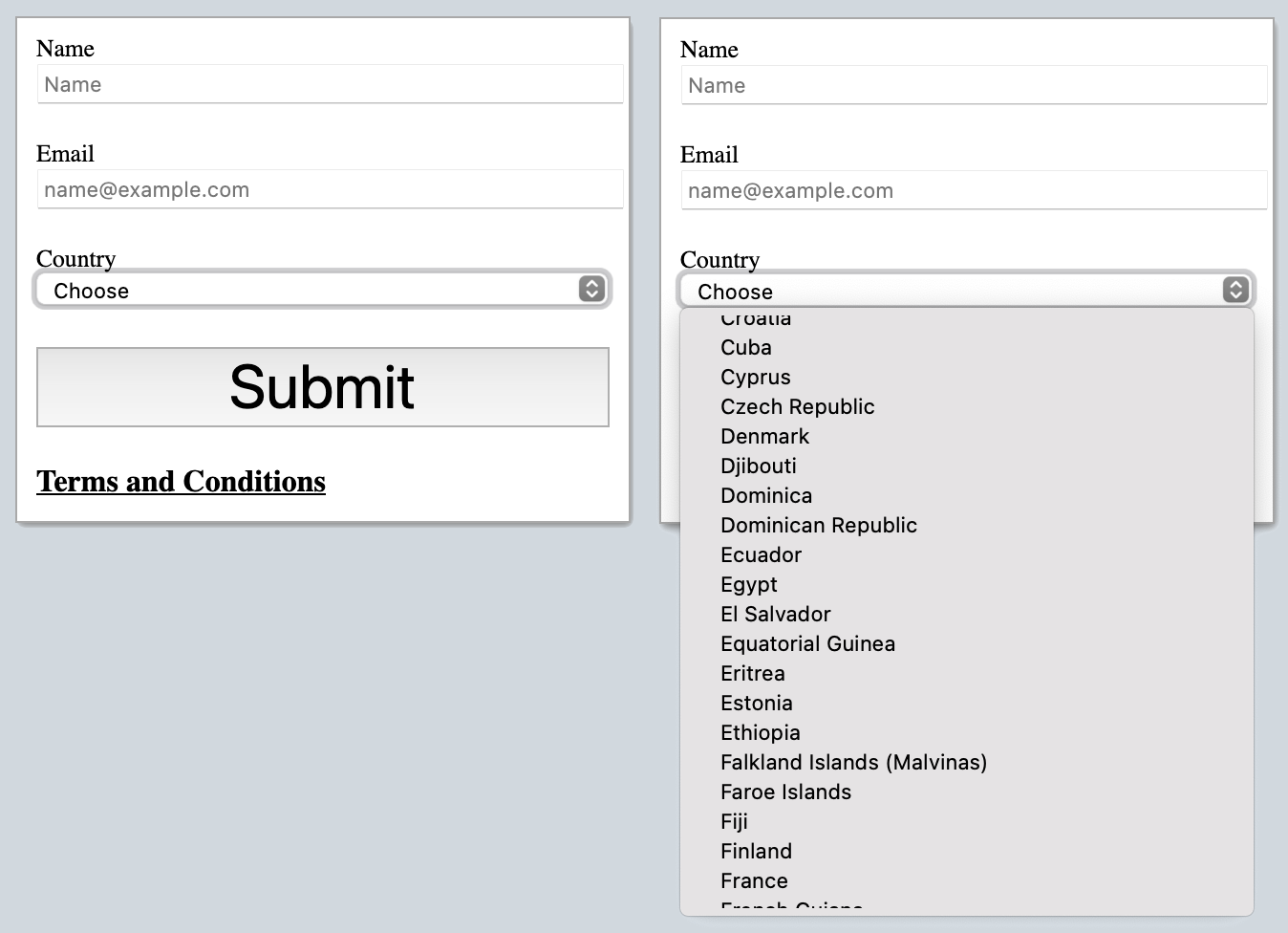
Figure 19 shows an example of a very simple GUI of a subscription application. The root of the widget tree is a form. This form contains several widgets for users to enter their information: text boxes for the name and email, a combobox to select the country, a submit button and a link. The combobox on its side contains a menu whose children are items corresponding to each possible selection. Initially, the Name text box has as properties: width = 300, height = 15, placeholder = "Name" and text = "". After a user enters her name, then the text property changes with the corresponding value. The same goes for the rest of the widgets.
GUI tests are a form of system tests, as they execute the entire application. They are designed from the user’s perspective. In general terms, a GUI test initializes the system under test, performs a series of GUI actions and then, it checks if the GUI state is correct.
For our small GUI a test case could be designed as following:
-
Open the subscription form
-
Enter "Jane Doe" in Name
-
Enter "jave@example.com" in Email
-
Select "Canada" in Country
-
Click Submit
-
Expect success message
This test checks that a user, entering the right information, is able to subscribe to the system. A test checking if the application detects an error in the data, for example, that the email is valid would do the following:
-
Open the subscription form
-
Enter "Jane Doe" in Name
-
Enter "not an email" in Email
-
Click Submit
-
Expect an error under Email
In general, GUI tests should verify that the required information is visible in the screen, that the position and size of the widgets is correct, that the appropriate error messages are shown at the right time and that the application does not crash or closes unexpectedly.
As with the rest of tests, manually executing GUI tests is tedious an extremely error prone, so we need to automate their execution. There are four main approaches to GUI test automation, all with their pros and cons:
- Capture and replay
-
Tests are executed manually once and a specialized tool records the actions performed by the user. Then, the tests can be executed as many times as we want and the result should be the same. This is a simple option to automate GUI tests that do not require testers to have programming skills. On the other side this form of test is highly sensitive to GUI changes. Any small modification to the interface renders the tests invalid and they have to be recreated again.
- Develop test scripts
-
We can develop scripts that emulate user actions and query the GUI state. This approach requires programming skills and it is arguably the most appealing for developers. There are plenty of libraries, frameworks and even domain specific languages (DSLs) to develop GUI test scripts for desktop, web and mobile applications, being Selenium one of the most used for the web. These tests can be usually integrated with testing frameworks like JUnit. As with other forms of tests, these have to be maintained and changed whenever the GUI changes. Listing 79 shows an implementation of a test verifying that the application shows an error if the user forgets to enter the name. It uses Selenium combined with JUnit and Hamcrest.
Listing 79. A simple Selenium test checking that the application shows an error if the user forgets to specify the name.@Test public void testMissingName() { String url = "http://localhost:5000"; WebDriver driver = new ChromeDriver(); driver.get(url); (1) driver.findElement(By.id("email")).sendKeys("jane@example.com"); (2) Select countrySelector = new Select(driver.findElement(By.id("country"))); (3) countrySelector.selectByValue("Canada"); (4) driver.findElement(By.id("submit")).click(); (5) List<WebElement> errors = driver.findElements(By.className("error")); (6) assertThat(errors, hasSize(1)); (7) }1 Go to the address where the application is deployed. 2 Find the email text box and fill it with jave@example.com.3 Find the combobox for the country. 4 Enter Canadaas the country value.5 Find and click the Submitbutton.6 Find error elements in the page. 7 Check that there is at least one error element. However, the code of this test is hard to follow, as it contains many GUI queries cluttering its actual intent. This particular test is also tangled with the GUI design. For example, errors are discovered by finding HTML elements with an
errorclass. If the GUI design changes, we need to change this part of the code in all tests doing the same. Therefore we need to find a way to develop these tests so they have a simpler code and are robust to changes. We shall discuss the Page Object Model (84) pattern for this matter. - Visual scripts
-
An interesting alternative to test scripts. The widgets participating in the tests are specified using images from screen captures of the application. The test execution uses image recognition techniques to detect the position of the widgets. EyeAutomate provides a set of tools to achieve this. While it is a simple alternative to put into practice, it still requires a sophisticated machinery underneath and it is still highly sensitive to GUI changes.
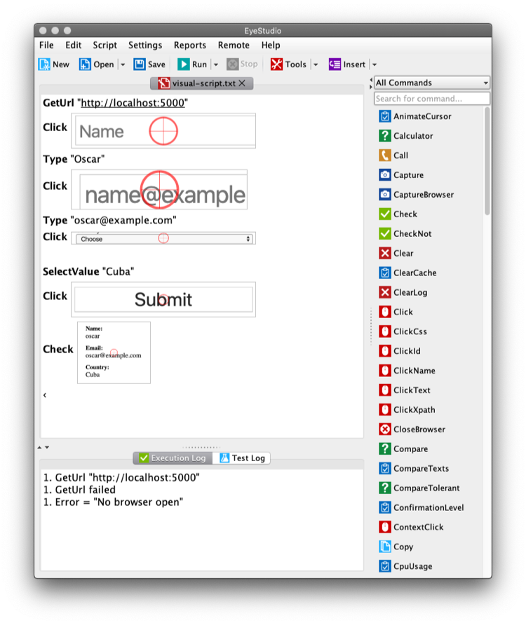 Figure 20. EyeAutomate script
 - Automated GUI testing
-
In the previous section we saw that we can automatically generate interesting test inputs and even test code. GUI tests are not an exception on that. Automating the GUI testing process requires a way to obtain the GUI state and the possible GUI actions. This allows to execute the application and automatically decide a sequence of actions to perform and a way to check the consistency of the GUI state. This can be seen as a type of fuzzing directed to the user actions as the input domain of the application. Test* implements this idea and automatically check the robustness of applications against random actions.
In the remaining sections we shall discuss how to write our GUI tests with the help of Selenium and how tools like Test* achieve GUI test automation.
5.1. Writing test scripts
Listing 79 shows an example of a test written with Selenium to check the response of the subscription form when the user forgets to enter her name.
Selenium is a set of libraries and tools designed to automate the interaction with web browsers. Although it is widely used for testing, it can be employed in many other automation tasks. Its core functionalities are based on the WebDriver, an API that makes possible to inspect remotely control browsers by emulating user actions and allows code to inspect the content presented by the browser. Other alternatives like Puppeteer do the same based on the Chrome DevTools protocol.
Concrete WebDrivers are specific to each browser, but the API is general enough so the code we write works no matter the browser we are using. In [simple-selenoum-test] we can notice that it is possible to search for web elements using their identifiers By.id or style class name By.className. We see that we can send keyboard input with sendKeys, select an element with selectByValue and even click on web page elements. The functionalities of Selenium go way beyond this basic operations as they permit to inspect every aspect of the web page and to build more complex interactions like drag and drops.
Suppose we want to write a similar test case for our application to verify the scenario in which the user forgets to enter the country. The code will be pretty much the same as before. But we know applications change in time. In particular, the GUI changes to improve the user experience, make the application more appealing or because we are incorporating a new framework with better user controls.
If, for example, we decide to show errors differently, or we decide to change the way the country is selected, then we have to change the code of all test cases we wrote this way. The GUI changed but the requirements are the same: there should be an error when the user forgets some of the form values. The test cases should be changed for technical reasons and tests should reflect more the requirements than the application implementation. Also, the GUI queries to obtain the visual elements are interweaved inside the test code. This makes the test case harder to read and understand. Its intent gets hidden by the machinery to build the tests.
The Page Object Model is a code design pattern that precisely aims at solving these two issues. Here we illustrate the pattern with a web application, but it could be used to test other forms of GUI as well.
5.1.1. Page Object Model
Page Object Model or simply Page Object is a design pattern that proposes to separate the test code from the page/GUI specific code (84). The main idea is to create classes to model each page in our application. These classes shall become the interface between the tests and the GUI. Page objects should allow the tests to do and see anything human users would do while providing a simple programming interface.
In a page object, any information exposed by the page, should become a property, any action a user can do should become a behavior or method of the class. This is an Object-Oriented approach to encapsulate GUI specific code and hide the structural complexity of the GUI. If the GUI changes, then only the page objects will change and not the test code. Listing 80 shows how the test case from Listing 79 could be written with a page object SubscribePage representing the subscription page. The SubscribePage has methods to emulate the possible actions: typeEmail, selectCountry and submit. It also has accessors to retrieve this information and the errors shown in the page.
@Test
public void testMissingName() {
    driver.get("http://localhost:5000");
    SubscribePage page = new SubscribePage(driver);
    page.typeEmail("jane@example.com")
            .selectCountry("Canada")
            .submit();
    assertThat(page.errors(), hasSize(1));
}
When creating page objects there is no need to represent the entire page, not even all pages in the application. We should focus on what is essential for testing. Doing otherwise will create an unnecessary burden as these objects have to be maintained. On the other hand, a page object may be composed by other page objects representing recurrent components in the application. Page objects should not contain assertions, so they can be reused among different tests, but they may include general purpose checks, for example, verify that the webdriver navigates the right page and that application the hasn’t crashed.
Let’s explore this pattern in a more complete example. We shall use Selenium from Java to test the Simba Organizer web application. This application is composed by a backend developed in Java using Quarkus and a frontend developed in TypeScript using Angular and third party libraries like PrimeNG and FullCalendar.
| Testing an Angular application from Java using Selenium is not the ideal option. However, it is feasible and the Java+Selenium stack can be applied to web applications developed in any other framework than Angular. For Angular applications the best choice is to use Protractor. |
Simba Organizer is a teaching project used in different student assignments at ISTIC, University of Rennes 1. It is a doodle-like application that allows a set of users to agree on the schedule of a meeting. One user creates an initial poll to decide the schedule of a meeting and proposes some time slots. Then the participants shall pick the option that best fits their availability and possibly send some comments. The application also interacts with services to create a shared pad for the meeting, to create a chatroom and to let users check their calendars when picking the time slot.
The workflow to create a poll for a meeting starts with a landing page shown in Figure 21. This page shows some instructions and the only action a user can do is to click the button at the bottom to start creating a poll. The actual poll creation page can be directly accessed, then modeling the landing page is not essential.
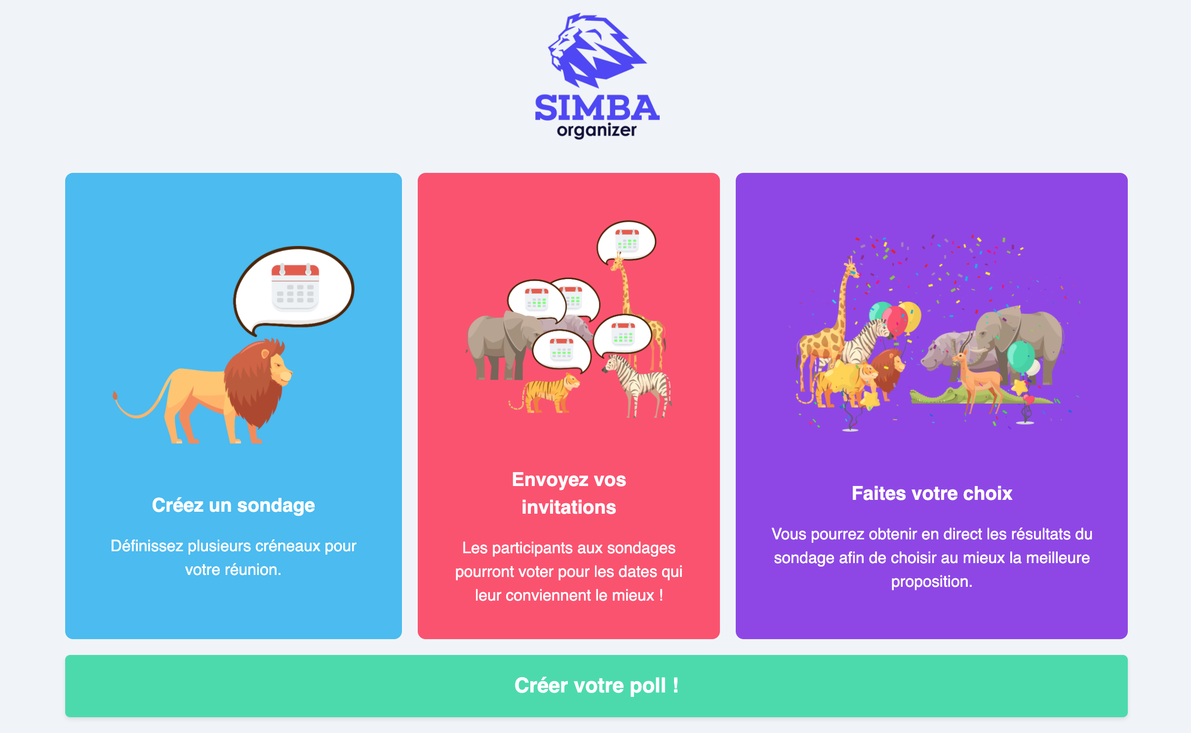
The poll creation page is shown in Figure 22. In this page a user must enter the general information of the meeting: mandatory title and place, optional description and whether the meeting will include a meal. Then, the user must click Next to move into the next creation step. If the user forgets one of the mandatory elements, then an error will be shown and the page will not change.
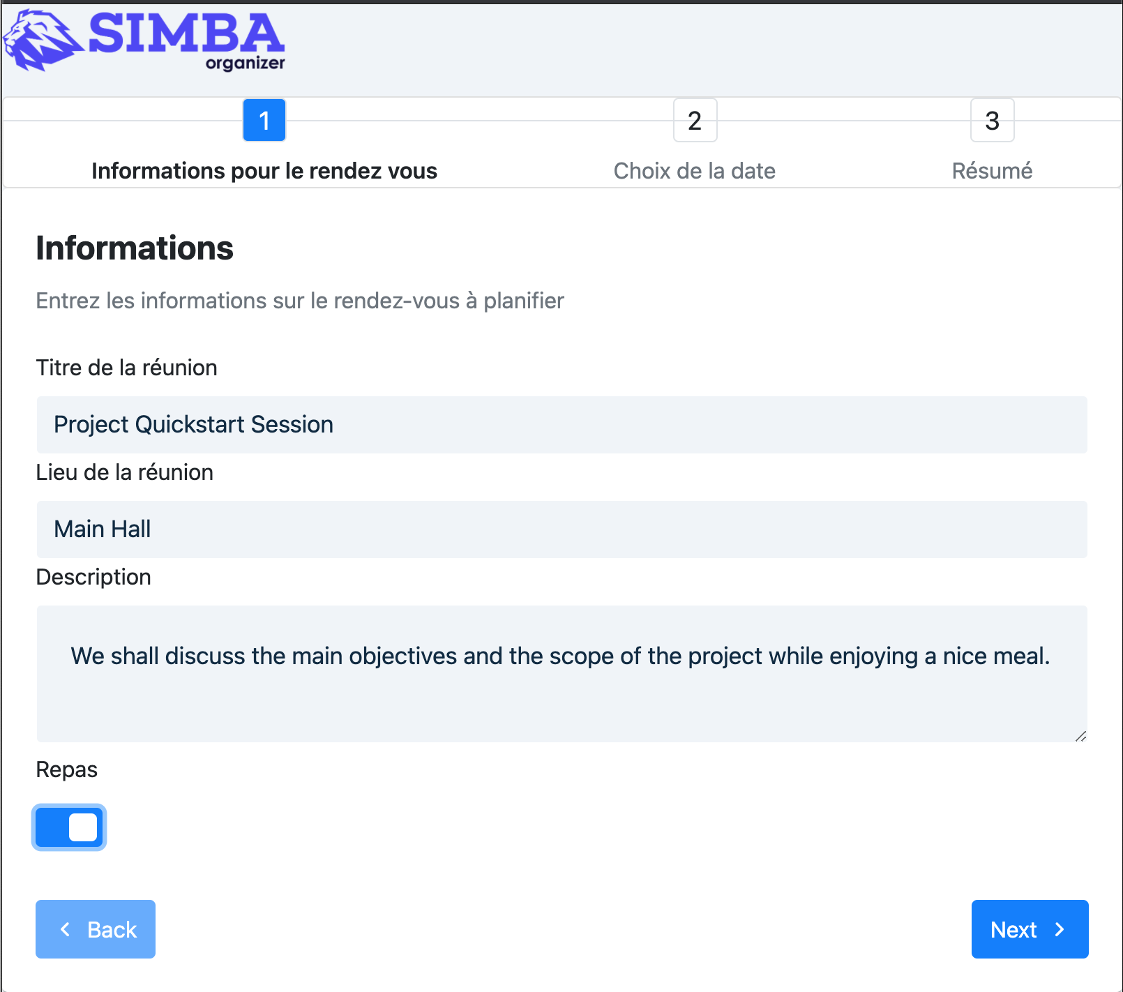
This page can be modeled by the class shown in Listing 81. The class has a constructor taking the WebDriver it should use to locate the web elements and interact with the browser. The class includes getter or accessor methods for all values shown in the form: title, place, description and hasMeal to know whether this value has been selected. In general, the accessor should be simple, they just find somehow the web element and returns the corresponding value. The result type of these methods should be as simple as possible: primitive types, string or simple data types. The goal is to reflect what is shown in the page and nothing more. Notice in the code how title was implemented: we use the driver to locate an input web element with id titre and then return the text value. Each action is represented as a method returning a page object. The implementation of typeTitle first finds the element and then instructs the browser to type the corresponding value. There may two possible outcomes when the user clicks Next: if there is an error the page does not change and error messages are shown. Otherwise the application shows the next step. We model these two scenarios with methods next and nextExectingErrors. Having two separate methods for this makes the test more readable and keeps the implementation simpler.
public class InformationPage {

    public InformationPage(WebDriver driver) { ... }

    public String title() {
        return driver.findElement(By.id("titre")).getText();
     }

    public InformationPage typeTitle(String value) {
        return driver.findElement(By.id("titre")).sendKeys(value);
     }

    public String place() { ... }

    public InformationPage typePlace(String value) { ... }

    public String description() { ... }

    public InformationPage typeDescription(String value) { ... }

    public boolean hasMeal() { ... }

    public InformationPage setHasMeal(boolean value) { ... }

    public List<String> errors() { ... }

    public DateselectionPage next() {
        driver.findElement(By.cssSelector("p-button[label=Next]")).click();
        return new DateselectionPage(driver);

    }

    public InformationPage nextExpectingErrors() {
        driver.findElement(By.cssSelector("p-button[label=Next]")).click();
        return this;
    }

}
In Listing 81 we have repeated driver.findElement queries several times. These can be avoided by simply having instance fields holding the right value and filling them in the construction. Selenium also provides some functionalities to make this simpler and more declarative using annotations. This is shown in Listing 82. We annotate fields with the corresponding element selectors and call PageFactory.initElements will handle their creation and assignment.
class InformationPage {

    private final WebDriver driver;

    @FindBy(id = "titre")
    private WebElement titleInput;

    @FindBy(css ="p-button[label=Next]")
    private WebElement nextButton;

    public InformationPage(WebDriver driver) {
        Objects.requireNonNull(driver);
        this.driver = driver;
        PageFactory.initElements(driver, this);
    }

    public String title() {
        return titleInput.getText();
    }

    public InformationPage nextExpectingErrors() {
        nextButton.click();
        return this;
    }

    ...
}
Once the user specifies the initial information of the meeting the application shows a page where she can select the initial options for the time slots. This page is shown in Figure 23. This page shows a calendar component where the user can create the time slots. It has also a switch the user can activate to enter a URL to an iCalendar feed so she can check her own time occupation. The user can move to the next stop at any time since it is not mandatory to set these initial options for the poll.
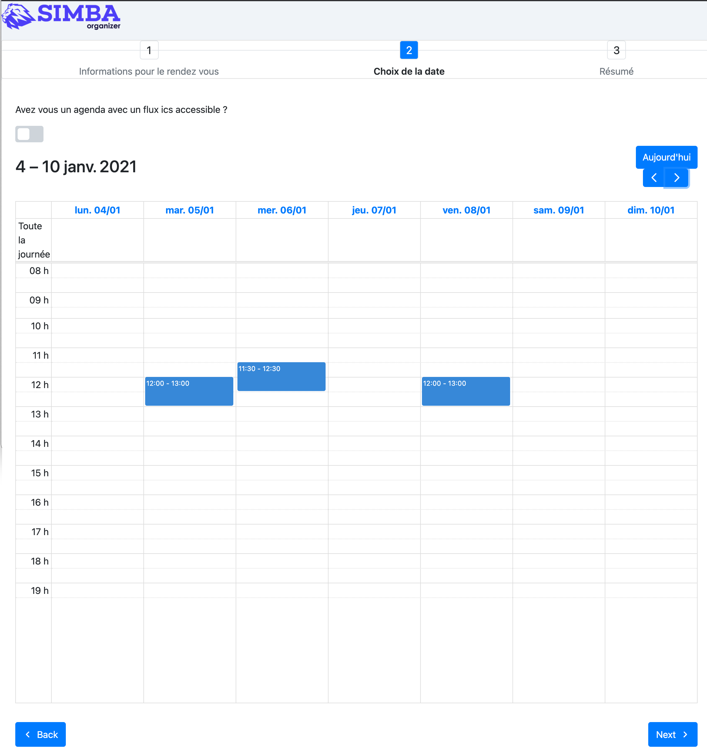
This page is particularly challenging for testing. On the one hand, the interaction with the calendar is rather complex. Users should click, drag and release the mouse to create an event in the calendar. Furthermore, users can even edit the events they have already created. On the other hand, fetching the iCalendar feed is an asynchronous operation which posses timing problems.
We should make page object models as simple as possible, since they must be updated each time the GUI changes. So, we should not aim at implementing all the calendar functionalities, besides, this a third party component that we may change at any time and we are not interested in testing it. At this point we assume it works correctly.
For the asynchronous operations we have not better solution than to wait until its result become visible. But also, we must set a reasonable timeout for the wait, so in case the operation fails and never sends back the results the test can also fail. These timeouts are often sources of flaky tests as we saw in previous sections so they must be handled with care.
Listing 83 shows how we can model this page. The purpose of this page is to select the initial time slot proposals. This is achieved with addOption. The method takes only the start and end LocalDateTime instances to create the slot. LocalDateTime is a class included in the java.time package. Inside, the method should interact with the calendar component to click in the right places. This may be hard. Since this is an Angular application we can also interact directly with the JavaScript code, which breaks a bit the encapsulation but might be simpler. There is no easy solution for this. However, implementing addOption hides all this complexity form the tests and makes the operation reusable. On its side, the options method returns the time slots we added to the calendar. Slot is a simple data class we created to represent a pair of start and end LocalDateTime.
public class DateSelectionPage {

    public DateSelectionPage(WebDriver driver) { ... }

    public boolean hasICS() { ... }

    public DateSelectionPage setHasICS(boolean value) { ... }

    public boolean isICSVisible() { ... }

    public String ICS() { ... }

    public DateSelectionPage typeICS(String value) { ... }

    public DateSelectionPage addOption(LocalDateTime start, LocalDateTime end) { ... }

    public List<Slot> options() { ... }

    public List<Slot> ICSEvents() { ... }

    public SummaryPage next() { ... }

    public InformationPage back() { ... }

}
If the user wants to consult her iCalendar, she must activate the switch, then a text box appears and she should enter the right URL there. Then, the events are fetched and shown in the calendar. All these operations are encapsulated in setHasICS to activate or deactivate the switch, isICSVisible to know if the text box is visible, ICS to get the value specified for the iCalendar URL, typeICS to set the value and ICSEvents to consult the events displayed in the calendar. Typing the iCalendar URL needs the text box to be visible. While the operation seems immediate after we activate the switch we have to be sure that the web element is visible. We can instruct the driver to wait for such things, Listing 84 shows how we can do that.
int timeout = 10;
WebDriverWait wait = new WebDriverWait(driver, timeout);
WebElement element = driver.findElement(By.id("ics"));
ExpectedCondition<Webelement> condition = ExpectedConditions.visibilityOf(element), timeout);
wait.until(condition);
The rest of the class is similar to the previous model: it has methods to access the information and method to go to the previous and next steps. When creating page object models it might be a good idea to have a base class, in which we can put all the common actions, for example, navigation methods, the waiting code and default timeouts. Then all the models we write can extend this base class.
After the poll has been created, the application displays a summary page shown in Figure 24.
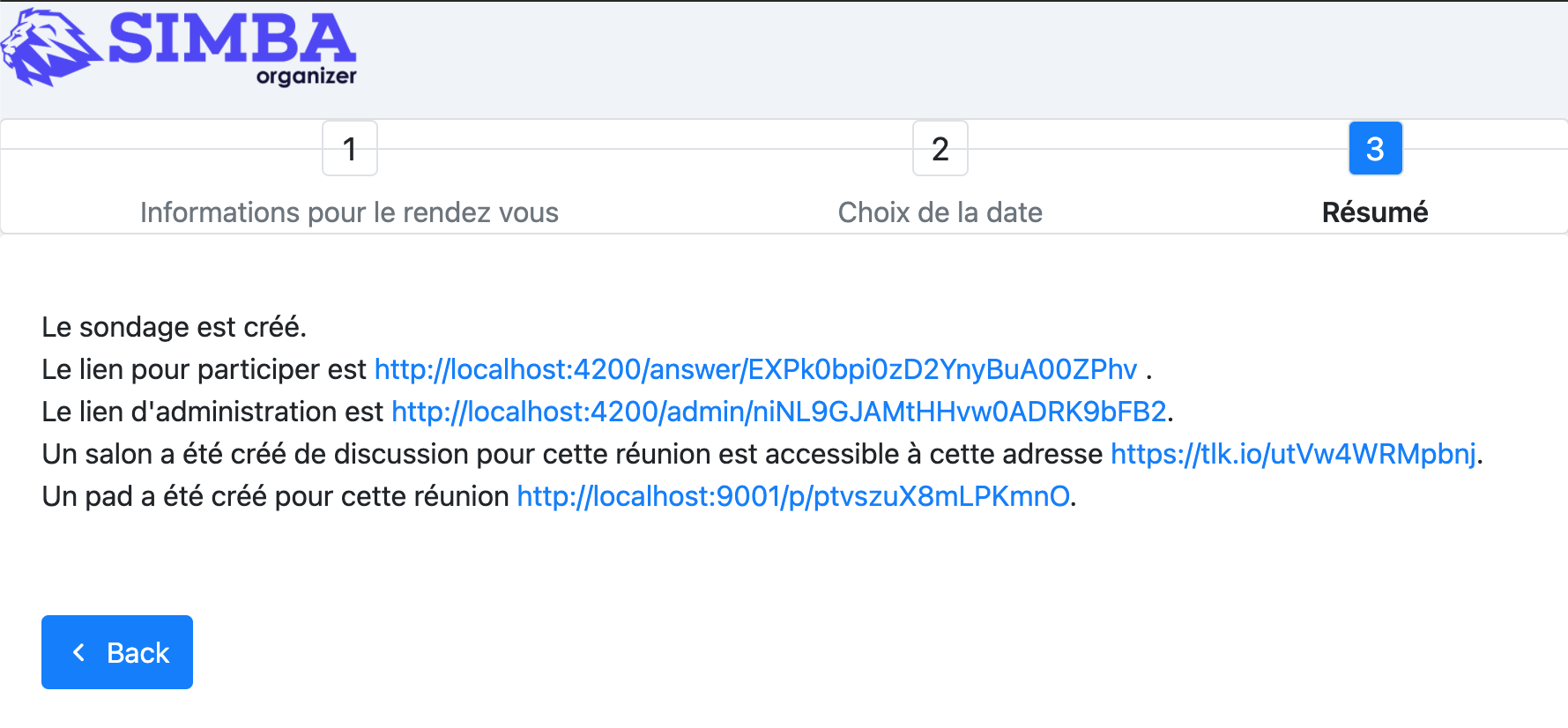
The model is simple, it just provides access to the URLs and method to navigate to the administration and participation pages. The chatroom and pad URLs are provided by third party services. We may opt not to create page object models for them or to create very simple classes to query the content of the pages to see if the information is correct, but nothing more since we do not want to test external components.
public class SummaryPage {

    public SummaryPage(WebDriver driver) { ... }

    public List<String> urls() { ... }

    public String participationURL() { ... }

    public String adminURL() { ... }

    public String chatRoomURL() { ... }

    public String padURL() { ... }

    public ParticipationPage navigateParticipationURL() { ... }

    public AdminPage navigateAdminPage() { ... }

    public DateSelectionPage back() { ... }

}
The poll administration page is shown in Figure 25. It shows the title, the place, if there is a meal planned for the meeting, comments from the participants, each option, and buttons to select the final option and close the poll. It also has links to create a new poll, to modify the existing poll, to go to the chatroom, the pad and even to share the poll. The model is shown in Listing 86. It is similar to the models before. The new aspect here is that we have modeled each option visual section as a different page object. This reduces the complexity of the AdminPage code.
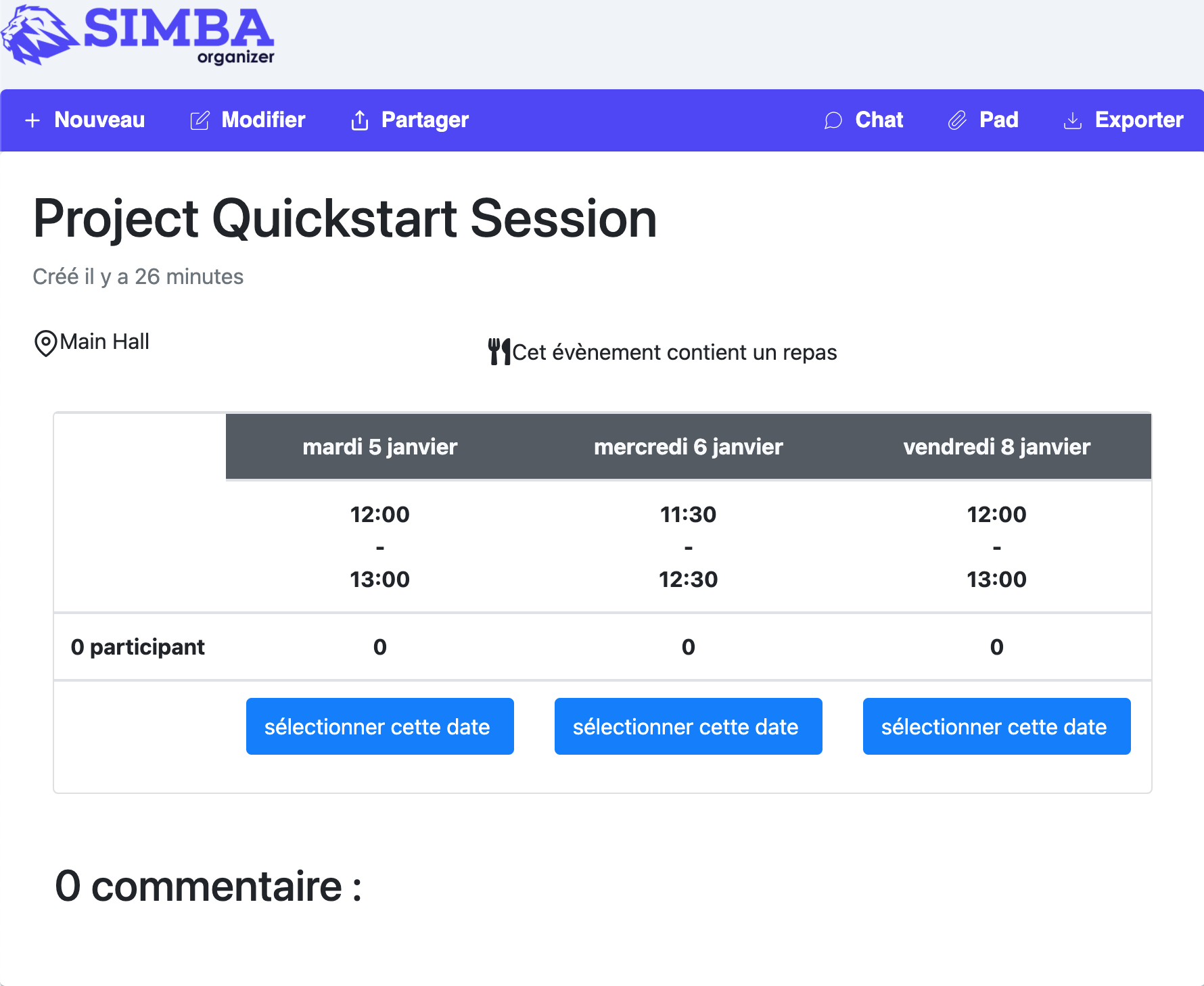
public class AdminPage {

    public AdminPage(WebDriver driver) { ... }

    public InformationPage createNew() { ... }

    public InformationPage modify() { ... }

    public String title() { ... }

    public String place() { ... }

    public boolean hasMeal() { ... }

    public List<String> comments() { ... }

    public List<OptionPanel> options() { ... }

    public String chatRoomURL() { ... }

    public String padURL() { ... }

    public String urlToShare() { ... }

}
The OptionPanel class is shown in Listing 87. It contains information about the start and end times and a method to select the option.
class OptionPanel {

    public LocalDateTime startsAt() { ... }

    public LocalDateTime endsAt() { ... }

    public AdminPage select() { ... }

}
With the models in place we can start writing test cases. Listing 88 shows a test case that checks if the application shows an error when the user forgets the title of the meeting.
@Test
void testNoTitleShowsAnError() {
    navigate(CREATE_URL);
    InformationPage page = new InformationPage(driver);
    page.typeDescription("We shall discuss very important matters while having a nice meal.")
            .typePlace("Very interesting place")
            .setHasMeal(true)
            .nextExpectingErrors()
    ;
    assertFalse(page.errors().isEmpty());
}
Listing 89 shows a test case verifying that the admin page displays the option selected during the creation of the poll. It is already a long test case that would be more complex without page objects.
@Test
void getTheOptions() {
    navigate(CREATE_URL);

    // Meeting information
    InformationPage information = new InformationPage(driver);
    information.typeTitle("Meeting").typePlace("Place");

    //Selecting options
    DateSelectionPage dateSelection = information.next();
    LocalDate nextWorkingDate = DateUtils.nextWorkingDay();
    LocalDateTime meetingStartsAt = LocalDateTime.of(nextWorkingDate, LocalTime.of(10, 0));
    LocalDateTime meetingEndsAt = LocalDateTime.of(nextWorkingDate, LocalTime.of(12, 0));
    dateSelection.addOption(meetingStartsAt, meetingEndsAt);

    // Navigating to the admin page
    SummaryPage summaryPage = dateSelection.next();
    AdminPage admin = summaryPage.navigateAdminPage();

    // Getting the list of options
    List<OptionPanel> options = admin.options();

    // Verifying that the option is displayed correctly
    assertEquals(1, options.size(), "Only one option must be available");
    OptionPanel option = options.get(0);
    assertEquals(meetingStartsAt, option.startsAt(), "Incorrect starting date/time");
    assertEquals(meetingEndsAt, option.endsAt(), "Incorrect ending date/time");

}
As with any solution the Page Object Mode design pattern may not fit every scenario. Its misuse may bring more harm than good. It is usually argued that page object models are hard to maintain and are not well documented (85). Like any other form of testing, GUI tests are subject to code smells, so we need to watch for code repetition, insufficient abstractions, and hard-to-understand code.
If a GUI has too much logic embedded, then implementing Page Object Model is challenging as the application becomes less testable. Development patterns like Model-View-Controller, Model-View-Presenter and Model-View-ViewModel or Passive View propose ways to organize the application code so the GUI has less logic and, as a result, it becomes easier to test. Also, interacting with the Controller, Presenter or the ViewModel can be easier than interacting directly with the visual elements (86).
5.2. Fully automated GUI testing
As said before, a GUI test initializes the system under test, performs a series of GUI actions and then it checks if the GUI state is correct. If we can automatically discover which actions can be done at any instant during the execution of a program and if we can automatically compare application states, then we can automatically generate GUI tests. In fact, if we consider the set of GUI/user actions as the input domain, we can fuzz graphical applications by generating random action sequences.
Test* (reads as Testar) is a research tool implementing an automated GUI random testing process. The general workflow is shown in Figure 26.
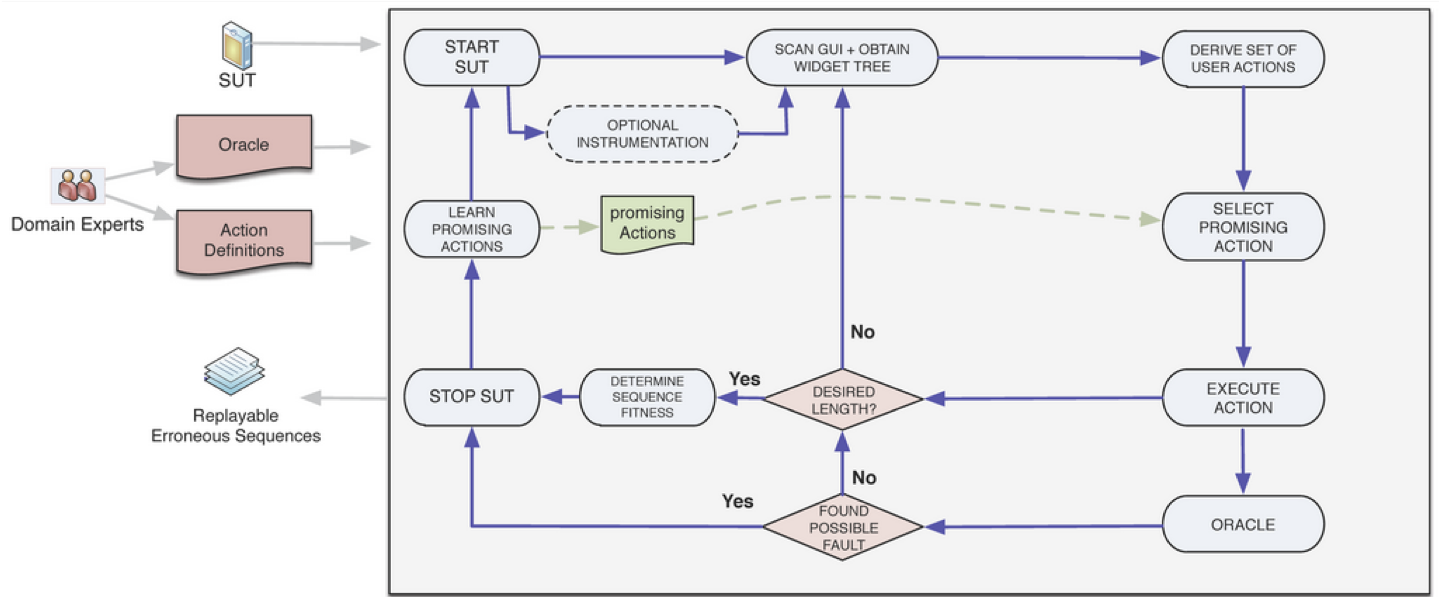
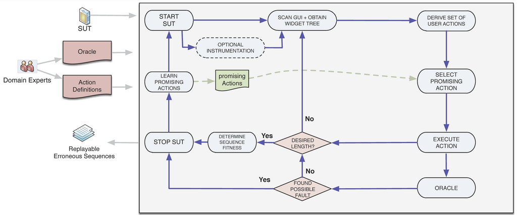
The process starts the System Under Test (SUT) and optionally instruments its code to obtain more information during the execution of user actions. Then, it scans the GUI to obtain sthe state, conformed by the widget tree and all their properties. Test* uses the accessibility API of the underlying operating system. This API provides direct access to the entire widget tree, their properties such as: their position, size, whether the widget is enabled or focused, and further attributes like text, title or any associated value. For example Figure 27 shows the set of properties the accessibility API provides for a button of the Calculator application in MacOS. Using the accessibility API, Test* can target any graphical application that respects the accessibility conventions.
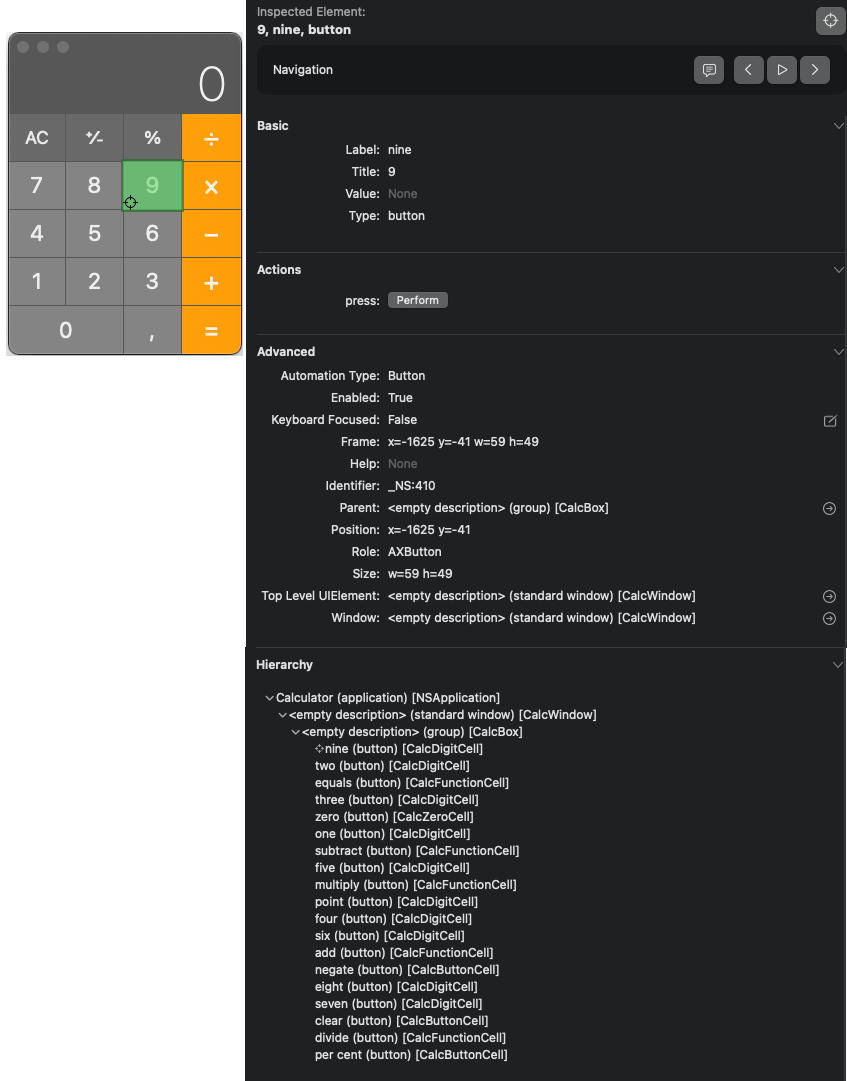
By inspecting the GUI state ,the tool is able to derive a set of possible actions. The tool automatically skips actions that are not meaningful like clicking on buttons that are hidden by other windows. The tool can also be configured with custom, more complex actions, targeting personalized widgets, and even actions to avoid, like closing the main window.
At each step, the tool randomly selects one of the identified actions. While this selection is random, the tool implements more intelligent mechanisms to identify action that are likely to trigger failures, such as actions that not executed often during the process. This action selection step can be customized as well. After the action has been selected, the state is updated and the process continues until some desired stopping conditions are met.
Each state reached by Test* is inspected for failures. By default, the tool checks implicit oracles similar to those we discussed for fuzzing like: the presence of application crashed and hangs. The tool also allows to specify other oracles like detecting error pop-ups from their messages or more complex assertions.
If a crash is found, then the whole action sequence to that point is stored with screenshots of the failure and the intermediate steps. Test* has been able to find actual critical failures in industry-level applications (87).
References
-
Andreessen, M. (2011). Why software is eating the world. Wall Street Journal, 20(2011), C2.
-
Wikipedia. Software Bug. https://en.wikipedia.org/wiki/Software_bug, Last accessed: 17/03/2020.
-
Ghahrai A. (2018). Error, Fault and Failure in Software Testing. https://www.testingexcellence.com/error-fault-failure-software-testing/ Last accessed: 17/03/2020.
-
Ammann, P., & Offutt, J. (2016). Introduction to software testing. Cambridge University Press.
-
Mancoridis S. Slides of his V&V course https://www.cs.drexel.edu/~spiros/teaching/SE320/slides/introduction.pdf)) Last accessed: 17/03/2020.
-
Moller, K-H., and Daniel J. Paulish. (1993). An empirical investigation of software fault distribution. Proceedings First International Software Metrics Symposium. IEEE (1993).
-
Fruhlinger J. (2017). What is the Heartbleed bug, how does it work and how was it fixed?. CSO (2017) https://www.csoonline.com/article/3223203/vulnerabilities/what-is-the-heartbleed-bug-how-does-it-work-and-how-was-it-fixed.html. Last accessed: 17/03/2020.
-
Slabodking G. (1998). Software glitches leave Navy Smart Ship dead in the water. GCN (1998) https://gcn.com/Articles/1998/07/13/Software-glitches-leave-Navy-Smart-Ship-dead-in-the-water.aspx Last accessed: 17/03/2020.
-
Arnold D. (2000). The Patriot Missile Failure. http://www-users.math.umn.edu/~arnold/disasters/patriot.html Last accessed 17/03/2020.
-
Hansell S. (1994). Glitch Makes Teller Machines Take Twice What They Give. https://www.nytimes.com/1994/02/18/business/glitch-makes-teller-machines-take-twice-what-they-give.html. Last accessed: 10/09/2018.
-
Jézéquel, J-M., and Bertrand Meyer. (1997). Design by contract: The lessons of Ariane. Computer 30.1 (1997): 129-130.
-
Ceguerra A. (2001). Software Bug Report: Mars Climate Orbiter Assignment 1 for Verification. http://courses.engr.uky.edu/ideawiki/data/media/classes/06c/585/mars_climate_orbiter.pdf. Last accessed: 17/03/2020
-
Johnson P. (2012). Curiosity about lines of code. https://www.itworld.com/article/2725085/big-data/curiosity-about-lines-of-code.html. Last accessed: 12/09/2018.
-
Turing, A. M. (1936). On computable numbers, with an application to the Entscheidungsproblem. J. of Math, 58(345-363), 5.
-
Lines of Code Linux Kernel.svg. https://commons.wikimedia.org/wiki/File:Lines_of_Code_Linux_Kernel.svg. Last accessed: 17/03/2020.
-
OpenSignal. (2015). Android Fragmentation. https://www.opensignal.com/sites/opensignal-com/files/data/reports/global/data-2015-08/2015_08_fragmentation_report.pdf). Last accessed: 17/03/2020.
-
Trikha R. (2020, Jul 2nd). The Inevitable Return of COBOL Published by Ritika Trikha https://blog.hackerrank.com/the-inevitable-return-of-cobol/. Last accessed: 06/07/2020.
-
CNBC, Reuters (2017, Apr 11th) Banks scramble to fix old systems as IT ‘cowboys’ ride into sunset https://www.cnbc.com/2017/04/11/banks-scramble-to-fix-old-systems-as-it-cowboys-ride-into-sunset.html. Last accessed: 06/07/2020.
-
Leswing K., CNBC (2020 Apr 6th) New Jersey needs volunteers who know COBOL, a 60-year-old programming language https://www.cnbc.com/2020/04/06/new-jersey-seeks-cobol-programmers-to-fix-unemployment-system.html. Last accessed: 06/07/2020.
-
Mittal, S. (2016). A survey of techniques for approximate computing. ACM Computing Surveys (CSUR), 48(4), 1-33.
-
Hardesty L. (2010). When good enough is better. MIT News Office. https://news.mit.edu/2010/situationally-award-0513 Last accessed: 28/10/2020.
-
Misailovic, S., Sidiroglou, S., Hoffmann, H., & Rinard, M. (2010, May). Quality of service profiling. In Proceedings of the 32nd ACM/IEEE International Conference on Software Engineering-Volume 1 (pp. 25-34).
-
Meyer, B. (2008). Seven principles of software testing. Computer, 41(8), 99-101. https://doi.org/10.1109/MC.2008.306 Also available here: http://se.inf.ethz.ch/old/people/meyer/publications/testing/principles.pdf
-
The Netflix Simian Army. (2011). https://netflixtechblog.com/the-netflix-simian-army-16e57fbab116 Last accessed: 01/05/2020
-
Continuous Integration. (2006). https://martinfowler.com/articles/continuousIntegration.html Last accessed: 01/05/2020
-
Continuous Integration. https://www.thoughtworks.com/continuous-integration Last accessed: 01/05/2020
-
Spinellis, D. (2006). Code quality: the open source perspective. Adobe Press.
-
Fowler M. (May 2019). Is High Quality Software Worth the Cost? https://martinfowler.com/articles/is-quality-worth-cost.html Last accessed: 22/04/2020
-
Boehm, B. W., Brown, J. R., & Lipow, M. (1976, October). Quantitative evaluation of software quality. In Proceedings of the 2nd international conference on Software engineering (pp. 592-605). IEEE Computer Society Press. https://dl.acm.org/citation.cfm?id=807736
-
ISO/IEC 25010:2011 Systems and software engineering — Systems and software Quality Requirements and Evaluation (SQuaRE) — System and software quality models. https://www.iso.org/standard/35733.html Last accessed: 22/04/2020
-
Google Java Style Guide https://google.github.io/styleguide/javaguide.html Last accessed: 28/10/2020
-
Oracle (1997). Java Code Conventions https://www.oracle.com/technetwork/java/codeconventions-150003.pdf Last accessed: 28/04/2020
-
Microsoft (2008). Names of Classes, Structs, and Interfaces https://docs.microsoft.com/en-us/dotnet/standard/design-guidelines/names-of-classes-structs-and-interfaces Last accessed: 28/04/2020
-
van Rossum G. (2001). Style Guide for Python Code https://www.python.org/dev/peps/pep-0008/ Last accessed: 29/04/2020
-
Wikipedia. Indentation style. https://en.wikipedia.org/wiki/Indentation_style Last accessed: 30/04/2020
-
Microsoft (2018). Secure coding guidelines. https://docs.microsoft.com/en-us/dotnet/standard/security/secure-coding-guidelines Last accessed: 30/04/2020
-
Google. Google Java Style Guide. https://google.github.io/styleguide/javaguide.html Last accessed: 30/04/2020
-
Forwler. M. (2006). CodeSmell https://martinfowler.com/bliki/CodeSmell.html Last accessed: 01/05/2020
-
Source Making. Code Smells https://sourcemaking.com/refactoring/smells Last accessed: 01/05/2020
-
Source Making. AntiPatterns. https://sourcemaking.com/antipatterns Last accessed: 30/04/2020
-
Glover A. (2006). Monitoring Cyclomatic Complexity. https://www.ibm.com/developerworks/library/j-cq03316/index.html Last accessed: 05/05/2020
-
McLoone J. (2012). Code Length Measured in 14 Languages https://blog.wolfram.com/2012/11/14/code-length-measured-in-14-languages/ Last accessed: 15/06/2020
-
McCabe, T. J. (1976). A Complexity Measure. IEEE Transaction on Software Engineering, vol SE-2(4).
-
Hummel B. (2014) McCabe’s Cyclomatic Complexity and Why We Don’t Use It. https://www.cqse.eu/en/news/blog/mccabe-cyclomatic-complexity/ Last accessed: 17/06/2020
-
Chidamber, S. R., & Kemerer, C. F. (1994). A metrics suite for object oriented design. IEEE Transactions on software engineering, 20(6), 476-493. Online: http://www.pitt.edu/~ckemerer/CK%20research%20papers/MetricForOOD_ChidamberKemerer94.pdf Last accessed: 18/06/2020
-
Fowler, M. (2001). Reducing Coupling. IEEE Softw., 18, 102-104. Online: https://martinfowler.com/ieeeSoftware/coupling.pdf Last accessed 18/06/2020
-
Ujhazi, B., Ferenc, R., Poshyvanyk, D., & Gyimothy, T. (2010, September). New conceptual coupling and cohesion metrics for object-oriented systems. In 2010 10th IEEE Working Conference on Source Code Analysis and Manipulation (pp. 33-42). IEEE.
-
Appleton B. Introducing Demeter and its Laws. http://www.bradapp.com/docs/demeter-intro.html Last accessed 18/06/2020
-
Martin, R. C., & Martin, M. (2006). Agile principles, patterns, and practices in C# (Robert C. Martin). Prentice Hall PTR. Online: https://ivanderevianko.com/wp-content/uploads/2013/10/Agile-Principles-Patterns-and-Practices-in-C.pdf Last accessed: 19/06/2020
-
Martin, R. (2014) The Single Responsibility Principle https://blog.cleancoder.com/uncle-bob/2014/05/08/SingleReponsibilityPrinciple.html Last accessed: 19/06/2020
-
Bieman, J. M., & Kang, B. K. (1995). Cohesion and reuse in an object-oriented system. ACM SIGSOFT Software Engineering Notes, 20(SI), 259-262.
-
Gamma, E., Helm, R., Johnson, R., & Vlissides, J. (1994). Design Patterns Elements of reusable object-oriented sofware. Addison Wesley.
-
Sadowski, C., Söderberg, E., Church, L., Sipko, M., & Bacchelli, A. (2018, May). Modern code review: a case study at google. In Proceedings of the 40th International Conference on Software Engineering: Software Engineering in Practice (pp. 181-190).
-
Aniche M. and others, The Testing Pyramid. Software Testing from Theory to Practice. https://sttp.site/chapters/pragmatic-testing/testing-pyramid.html Last accessed: 01/09/2020
-
Garousi, V., and Küçük, B. (2018). Smells in software test code: A survey of knowledge in industry and academia. Journal of Systems and Software, 138, 52-81. https://doi.org/10.1016/j.jss.2017.12.013
-
Meszaros G., Smith S.M., Andrea J. (2003) The Test Automation Manifesto. In: Maurer F., Wells D. (eds) Extreme Programming and Agile Methods - XP/Agile Universe 2003. XP/Agile Universe 2003. Lecture Notes in Computer Science, vol 2753. Springer, Berlin, Heidelberg. https://doi.org/10.1007/978-3-540-45122-8_9 Available online at: http://xunitpatterns.com/~gerard/xpau2003-test-automation-manifesto-paper.pdf
-
xUnitPatterns.com Assertion Roulette http://xunitpatterns.com/Assertion%20Roulette.html Last accessed: 07/09/2020
-
Micco J. (2016) Flaky Tests at Google and How We Mitigate Them https://testing.googleblog.com/2016/05/flaky-tests-at-google-and-how-we.html Last accessed: 10/09/2020
-
Li, N., & Offutt, J. (2016). Test oracle strategies for model-based testing. IEEE Transactions on Software Engineering, 43(4), 372-395.
-
Comar, C., Guitton, J., Hainque, O., & Quinot, T. (2012, February). Formalization and comparison of MCDC and object branch coverage criteria.
-
DeMillo, R. A., Lipton, R. J., & Sayward, F. G. (1978). Hints on test data selection: Help for the practicing programmer. Computer, 11(4), 34-41.
-
Coles, H., Laurent, T., Henard, C., Papadakis, M., & Ventresque, A. (2016, July). Pit: a practical mutation testing tool for java. In Proceedings of the 25th International Symposium on Software Testing and Analysis (pp. 449-452).
-
Coles, H. (2018, October). Making Mutants Work For You or how I learned to stop worrying and love equivalent mutants, Paris JUG October 24th 2018
-
Deng, L., Offutt, J., & Li, N. (2013, March). Empirical evaluation of the statement deletion mutation operator. In 2013 IEEE Sixth International Conference on Software Testing, Verification and Validation (pp. 84-93). IEEE.
-
Untch, R. H., Offutt, A. J., & Harrold, M. J. (1993, July). Mutation analysis using mutant schemata. In Proceedings of the 1993 ACM SIGSOFT international symposium on Software testing and analysis (pp. 139-148).
-
Arguelles, C., Ivanković, M., Bender, A., (2020, August) Code Coverage Best Practices. Available at https://testing.googleblog.com/2020/08/code-coverage-best-practices.html Last accessed: 12/11/202
-
Ivanković, M., Petrović, G., Just, R., & Fraser, G. (2019, August). Code coverage at Google. In Proceedings of the 2019 27th ACM Joint Meeting on European Software Engineering Conference and Symposium on the Foundations of Software Engineering (pp. 955-963).
-
Massol, V., (2013) Tip: Find out max Clover TPC for Maven modules Available at: https://massol.myxwiki.org/xwiki/bin/view/Blog/MaxCloverTPCTip Last accessed: 12/11/2020
-
Petrović, G., & Ivanković, M. (2018, May). State of mutation testing at google. In Proceedings of the 40th international conference on software engineering: Software engineering in practice (pp. 163-171).
-
Freeman S. (2007, April) Test Smell: Everything is mocked Available online: http://www.mockobjects.com/2007/04/test-smell-everything-is-mocked.html Last accessed: 23/11/2020
-
Day B. (2014) Better Unit Tests through Design Patterns: Repository, Adapter, Mocks, and more…. Available online: https://www.benday.com/wp-content/uploads/2014/08/benday-agile-2014-unit-testing-v2.pdf Last accessed: 23/11/2020
-
Miller J. (2008) Patterns in Practice. Design For Testability. Available online: https://docs.microsoft.com/en-us/archive/msdn-magazine/2008/december/patterns-in-practice-design-for-testability Last accessed: 23/11/2020
-
Moore J. (2019, September) Designing for testability. Available online: https://jenniferplusplus.com/designing-for-testability/ Last accessed: 23/11/2020
-
Source Making. Design patterns https://sourcemaking.com/refactoring/smells Last accessed: 23/11/2020
-
Beck, K. (2003). Test-driven development: by example. Addison-Wesley Professional.
-
Li, C. (2018, May) Why TDD is Bad (and How to Improve Your Process) Available online: https://medium.com/@charleeli/why-tdd-is-bad-and-how-to-improve-your-process-d4b867274255 Last accessed: 24/11/2020
-
Fox, C. (2019, November) Test-Driven Development is Fundamentally Wrong. Available online: https://hackernoon.com/test-driven-development-is-fundamentally-wrong-hor3z4d Last accessed: 24/11/2020
-
Schranz, T. (2014, January) A Case against Test-Driven Development. Available online: https://medium.com/product-love/a-case-against-test-driven-development-b230ebecee64 Last accessed: 24/11/2020
-
Gunnerson, E. (2017, November) #NoTDD Available online: https://docs.microsoft.com/en-us/archive/blogs/ericgu/notdd Last accessed: 24/11/2020
-
Forwler, M. (2014), Is TDD dead? Available online: https://martinfowler.com/articles/is-tdd-dead/ Last accessed: 24/11/2020
-
Zeller, A., Gopinath, R., Böhme, M., Fraser, G., & Holler, C. (2019). The fuzzing book.
-
Hamidy, G. (2020). Differential Fuzzing the WebAssembly https://aaltodoc.aalto.fi/handle/123456789/46101 Last accessed 28/12/2020
-
Nilizadeh, S., Noller, Y., & Pasareanu, C. S. (2019, May). DifFuzz: differential fuzzing for side-channel analysis. In 2019 IEEE/ACM 41st International Conference on Software Engineering (ICSE) (pp. 176-187). IEEE.
-
Moroz, M. (2019) AFL Technical details https://github.com/google/AFL/blob/master/docs/technical_details.txt Last accessed: 28/12/2020
-
Zalewski M. (2015) afl-fuzz: making up grammar with a dictionary in hand https://lcamtuf.blogspot.com/2015/01/afl-fuzz-making-up-grammar-with.html Last accessed: 28/12/2020
-
Fowler, M. (2013) Page Object https://martinfowler.com/bliki/PageObject.html Last accessed: 02/01/2021
-
Bahmutov, G. (2019) Stop using Page Objects and Start using App Actions https://www.cypress.io/blog/2019/01/03/stop-using-page-objects-and-start-using-app-actions/#page-objects-problems Last accessed: 03/01/2021
-
Fowler, M. (2006) Passive View https://martinfowler.com/eaaDev/PassiveScreen.html Last accessed: 03/01/2021
-
Rueda, U., Vos, T. E., Almenar, F., Martínez, M. O., & Esparcia-Alcázar, A. I. (2015). TESTAR: from academic prototype towards an industry-ready tool for automated testing at the user interface level. Actas de las XX Jornadas de Ingeniería del Software y Bases de Datos (JISBD 2015), 236-245.